As every September approaches, I can count on a series of spreadsheet questions. One popular Excel tutorial request is, “how do you look up a value on one Excel worksheet and use it on another Excel worksheet?”. For example, you need to translate a product number into a product name. One of my favorite Excel features is the VLOOKUP function and it can help with this task. (See Resources section at the end for a video tutorial and sample worksheets.)

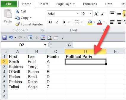
A recent case involved some voter registration data I needed to analyze. On one Excel spreadsheet, the voter’s party was listed as an alphanumeric value called “Pcode” and not the political party. This coding wasn’t intuitive. For example, “D” was for “American Independent Party”, but some thought it meant “Democratic Party”.

Non-intuitive column needing a lookup

One way to solve this problem is to create a worksheet with the Pcode and translation and have Excel use the VLOOKUP function for the party name. You might think of VLOOKUP as an Excel translator. I could then add a column called “Political Party” to my original worksheet to show the information from a lookup table.

Creating a Lookup Table

A lookup table includes the values you wish to “lookup” such as our Pcode and the translation such as a political party. You can place this table on the same worksheet, but for this Excel tutorial I added a worksheet called “Party Codes”.

Using the Starting VLOOKUP Example File,

1. Download the starting Excel sample file. The file link is also at the bottom of this tutorial.
2. Review Worksheet 1 called “Voters”. It has voter first and last names, but only a PCODE.
3. Review Worksheet 2 called “Party Codes”. It has a listing of party codes and political names. Each of the Party Codes and Names are unique. You’ll also note that Column A is in ascending order.

Worksheet with Translated Code Names

Using the Function

Excel’s VLOOKUP function uses 4 pieces of information. The function panel may seem intimidating with the terms, but it’s simpler than it looks.

To lookup a value using VLOOKUP,

1. Add your new column on the Voters worksheet that will display the info pulled from the Lookup table on Party Codes. In my example, I added a column called Political Party in Column D. This is where I will insert the Excel function.

Add a new Excel column for lookup values

1. Place your cursor in the first blank cell in that column. In my example, this is cell D2.
2. From the Formulas tab, select Insert Function. The Insert Function dialog will appear.

Inserting the VLOOKUP function

1. In the Search for a function: text box, type “vlookup” and click Go.
2. Highlight VLOOKUP and click OK.

Defining the Values

After you click OK, Excel’s Function Arguments dialog appears and allows you to define the four values. You’ll see that your starting cell and the formula bar show the beginning part of the function =VLOOKUP(). The Function Arguments dialog adds the needed data elements that will display between ().

For illustration purposes, I have overlaid the Party Codes worksheet on top to show the relationships.

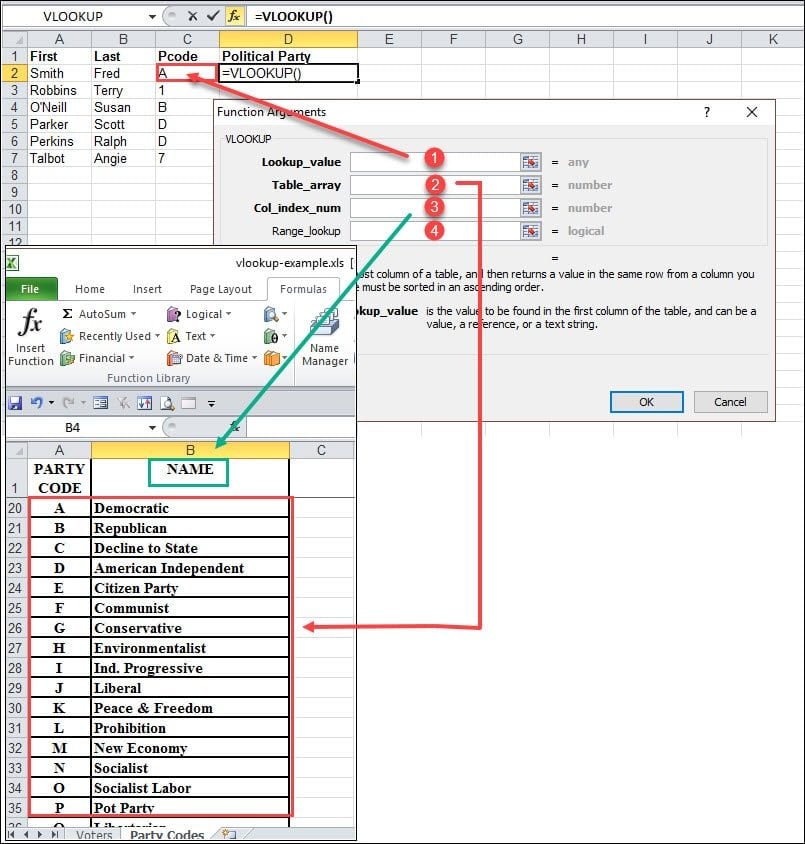
Mapping the VLOOKUP Function Arguments

1. Lookup_value – Think of this field as your starting point. In my example, I’ll click cell C2 so the value is filled in the dialog. I’m requesting Excel take the value of C2, which displays as the Pcode of “A” and find the matching political party on my lookup table on the Party Codes worksheet.

2. Table_array – This is the range for your lookup table. The range can be on your existing worksheet or another worksheet such as our “Party Codes”. When you click another worksheet and define the range, Excel prepends that tab name to the range such as ‘Party Codes’. In our case, I clicked the Party Codes worksheet and selected the range A2:B45.

3. Col_index_num – This is the number of the column on your lookup table that has the information you need. In our example, we want column 2 from the Party Codes worksheet which has the NAME of the political party.

4. Range-lookup – this field defines how close a match should exist between your Lookup_value (C2) and the value in the leftmost column on our lookup table. In our case, we want an exact match so we’ll use “FALSE”.

After clicking various cells, my dialog looks like the example below.

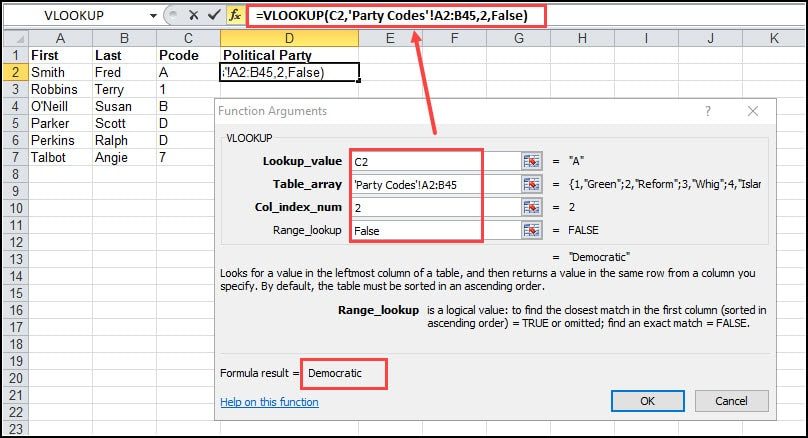
Mapped Values from Both Worksheets

You can see in the red outlined formula bar above, I now have more information based on my entries in the Function Arguments dialog box.

The other item of interest is that when you build these functions, Excel displays the result in the Formula result = text line. This is great feedback which can show if your function is on target. In our example, we can see Excel looked up the Pcode of “A” and returned the Political Party “Democratic”.

Copying the VLOOKUP Function to Other Cells

It doesn’t make sense to use VLOOKUP for one cell in your Excel spreadsheet. Instead, I want to copy the function to other cells in the same column.

To copy VLOOKUP to other column cells,

1. Click the cell containing the VLOOKUP arguments. In our example, this would be D2.
2. Make sure you changed your Table_array entry per Rule 3 above – Party Codes’!$A$2:$B$45.
3. Grab the cell handle that displays in the lower right corner.
4. Left-click and drag down the cell handle to cover your column range. You can also double-click the bottom-right corner of the fill handle.

Note: If I hadn’t changed to absolute reference as mentioned in Rule 3, I would’ve seen my table array entry shift by one cell as we dragged down through the other cells.

VLOOKUP is a powerful Excel function that can leverage spreadsheet data from other sources. There are many ways you can benefit from this function. In this example, I used a 1:1 code translation, but you could also use it for group assignments. For example, you could assign state codes to a region such as CT, VT, and MA to a region called “New England”. And for the adventurous, you can use VLOOKUP in your Excel formulas.

If you’re trying to a do a horizontal lookup, you’ll be happy to learn that Excel has a function for that called HLOOKUP. I haven’t done a HLOOKUP tutorial here, but there is a good one over at Deskbright I’d suggest you read.