Notes
Proof assistant
Four color theorem
In mathematics, the four color theorem, or the four color map theorem, states that no more than four colors are required to color the regions of any map so that no two adjacent regions have the same color. Adjacent means that two regions share a common boundary of non-zero length (i.e., not merely a corner where three or more regions meet). It was the first major theorem to be proved using a computer. Initially, this proof was not accepted by all mathematicians because the computer-assisted proof was infeasible for a human to check by hand. The proof has gained wide acceptance since then, although some doubts remain.
The theorem is a stronger version of the five color theorem, which can be shown using a significantly simpler argument. Although the weaker five color theorem was proven already in the 1800s, the four color theorem resisted until 1976 when it was proven by Kenneth Appel and Wolfgang Haken. This came after many false proofs and mistaken counterexamples in the preceding decades.
The Appel-Haken proof proceeds by analyzing a very large number of reducible configurations. This was improved upon in 1997 by Robertson, Sanders, Seymour, and Thomas who have managed to decrease the number of such configurations to 633 – still an extremely long case analysis. In 2005, the theorem was verified by Georges Gonthier using a general-purpose theorem-proving software.
Esquisse d’un Programme
Pareto principle
Regression toward the mean
In statistics, regression toward the mean (also called reversion to the mean, and reversion to mediocrity) is the phenomenon where if one sample of a random variable is extreme, the next sampling of the same random variable is likely to be closer to its mean. Furthermore, when many random variables are sampled and the most extreme results are intentionally picked out, it refers to the fact that (in many cases) a second sampling of these picked-out variables will result in “less extreme” results, closer to the initial mean of all of the variables.
Mathematically, the strength of this “regression” effect is dependent on whether or not all of the random variables are drawn from the same distribution, or if there are genuine differences in the underlying distributions for each random variable. In the first case, the “regression” effect is statistically likely to occur, but in the second case, it may occur less strongly or not at all.
Regression toward the mean is thus a useful concept to consider when designing any scientific experiment, data analysis, or test, which intentionally selects the “most extreme” events – it indicates that follow-up checks may be useful in order to avoid jumping to false conclusions about these events; they may be “genuine” extreme events, a completely meaningless selection due to statistical noise, or a mix of the two cases.[4
Prime number theorem
In mathematics, the prime number theorem (PNT) describes the asymptotic distribution of the prime numbers among the positive integers. It formalizes the intuitive idea that primes become less common as they become larger by precisely quantifying the rate at which this occurs. The theorem was proved independently by Jacques Hadamard and Charles Jean de la Vallée Poussin in 1896 using ideas introduced by Bernhard Riemann (in particular, the Riemann zeta function).
The first such distribution found is π(N) ~ N/log(N), where π(N) is the prime-counting function (the number of primes less than or equal to N) and log(N) is the natural logarithm of N. This means that for large enough N, the probability that a random integer not greater than N is prime is very close to 1 / log(N). Consequently, a random integer with at most 2n digits (for large enough n) is about half as likely to be prime as a random integer with at most n digits. For example, among the positive integers of at most 1000 digits, about one in 2300 is prime (log(101000) ≈ 2302.6), whereas among positive integers of at most 2000 digits, about one in 4600 is prime (log(102000) ≈ 4605.2). In other words, the average gap between consecutive prime numbers among the first N integers is roughly log(N).
Riemann hypothesis
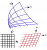
Curvilinear coordinates
In geometry, curvilinear coordinates are a coordinate system for Euclidean space in which the coordinate lines may be curved. These coordinates may be derived from a set of Cartesian coordinates by using a transformation that is locally invertible (a one-to-one map) at each point.