\sloppy

1 Eigenvalues and eigenvectors (from wikipedia)

1.1 Introduction

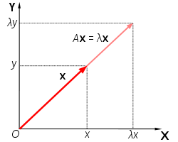
An eigenvector of square matrix A is a non-zero vector v that when the matrix is multiplied by v yealds a constant multiple of v, the multiplier being commonly dneoted by λthat is:

A⋅v = λ⋅v

The number λ is called the eigenvalue of A. In three-dimensional space an eigenvector v is arrow whose direction is eather preserved or exactly reversed after multiplication by A.

Figure 1.1 In this shear mapping the red arrow changes direction but the blue arrow does not. The blue arrow is an eigenvector of this shear mapping, and since its length is unchanged its eigenvalue is 1.

The corresponding eigenvalue determines how the length of the arrow is changed by the operation and wheather its direction is reversed or not, determined by whether the eigenvalue is negative or positive.

In abstract linear algebra these concepts are naturally extended to more general situations, where the set of real scalar factors is rplaced by any field of scalars (such as algebraic or coplex numbers); the set of Cartesean vectors ℜⁿis replaced by any vector space (such as continuous functions, the polynomials or the trigonometric series), and matrix multiplication is replaced by anay linear operator that maps vectorsto vectors (such as the derivate from calculus). In such case, the vector in eigenvector may be replaced by a mor speciffic term, such as „eigenfunction“,. Thus for example the exponential function f(x) = a^xis eigenfunction of the derivate operator „’“ with eigenvalue λ = ln(a) since its derivate is:

f^’(x) = (a^x)^’ = (e^x⋅ln(a))^’ = ln(a)⋅a^x = λ⋅f(x)

The prefix eigen- is adopted form german word eigen for „self-“ or „unique to“.

1.2 Eigenvectors and eigen values of a real matrix

Scalar vectors

u = ⎡⎢⎢⎢⎣ 1 3 4 ⎤⎥⎥⎥⎦, and v = ⎡⎢⎢⎢⎣ − 20 − 60 − 80 ⎤⎥⎥⎥⎦

A vector with thee elements, like u and v may represent a point in three-dimensional space, relative to some Cartesian coordinate system.

Figure 1.2 Marix A acts by stretching the vector x

If we multiplay any square matrix A with n rows and n columns by such vector v. The result wil be another vector w = A⋅v also with n rows and one column.

⎡⎢⎢⎢⎢⎢⎣ v₁ v₂ ⋮ v₃ ⎤⎥⎥⎥⎥⎥⎦is maped to

⎡⎢⎢⎢⎢⎢⎣ w₁ w₂ ⋮ w_n ⎤⎥⎥⎥⎥⎥⎦ = ⎡⎢⎢⎢⎢⎢⎣ A_1, 1 A_1, n A_n, 1 A_n, n ⎤⎥⎥⎥⎥⎥⎦⎡⎢⎢⎢⎢⎢⎣ v₁ v₂ ⋮ v_n ⎤⎥⎥⎥⎥⎥⎦

where for each i:

w_i = ⁿ⎲⎳_j = 1A_i, j⋅v_j

when w and v are paraler then v is eigenvector of A.\begin_inset Separator latexpar\end_inset

Example 1

A: = ⎡⎢⎣ 3 1 1 3 ⎤⎥⎦

In maple I got following eigenvalues

λ = ⎡⎢⎣ 4 0 0 2 ⎤⎥⎦

and following eigenvector

v = ⎡⎢⎣ 1 − 1 1 1 ⎤⎥⎦

Во чланакот од википедиаја

v = ⎡⎢⎣ 4 − 4 ⎤⎥⎦; A.v = ⎡⎢⎣ 8 − 8 ⎤⎥⎦ = 2.⎡⎢⎣ 4 − 4 ⎤⎥⎦ = λ⋅v

MMV. Може да го добиеш истово што го кажуваат во чланакот на Wikipedija со користење на опцијата output=list во командата Eigenvector()

На овој начин научив уште еден eigenvalue и eigenvector за оваа матрица (Maple):

4, ⎡⎢⎣ 1 1 ⎤⎥⎦

Всушност иницијалната форма на решение без output=list опцијата на Eigenvector() командата се содржани сите решенија 4 оди со ⎡⎢⎣ 1 1 ⎤⎥⎦, а 2 оди со ⎡⎢⎣ − 1 1 ⎤⎥⎦.

Example 2

A = ⎡⎢⎢⎢⎣ 1 2 0 0 2 0 0 0 3 ⎤⎥⎥⎥⎦

λ = ⎡⎢⎢⎢⎣ 3 0 0 0 1 0 0 0 2 ⎤⎥⎥⎥⎦

v = ⎡⎢⎢⎢⎣ 0 1 2 0 0 1 1 0 0 ⎤⎥⎥⎥⎦

Значи имајќи го во предвид решението од Wikipedia истото се добива со една команда. 3 оди со v_:, 1, 1 оди со v_:, 2 и 2 оди со v_:, 3.

1.2.1 Тривијални кејсови

The identity matrix I maps every vector to itself. Therefore, every vector is an eigen vector of I , wiht eigen value 1.

More generaly, if A is diagonal matrix the eigenvalues of a diagonal matrix are the elements of its main diagonal.

1.3 General definition

The concept of eigenvectors and eigenvalues extends naturally to abstract linear transformations on abstract vector spaces. Namely, let V be any vector space over some field K of scalars, and let T be a linear trasformation mapping V into V. We say that a non-zero vector v of V is eigenvector of T if (and only if) there is scalar λ in K such that:

T(v) = λ⋅v

This equation is called eigenvalue equation for T, and the scalar λ is eigenvalue of T coresponding to the eigenvector v. T(v) means the result of applying the operator T to the vector v. The marrix-specific definition is a special case of this abstract definition. Namely, the vector space V is the set of all column vectors of certain size nx1, and T is the linear transformation that consist in multiplying, a vector by the given n x n matrix A.

Some authors allow v to be the zero vector in definition of eigenvector.

1.4 Eigenspace and spectrum

If v is eigenvector fo T, with eigenvalue λ, then any scalar multiple α⋅v of v with nonzero α is also an eigenvector with eigenvalue λ, since

T(αv) = α T(v) = α(λv) = λ(αv)

Moreover, if u and v are eigenvectors with the same eigenvalue then u + v is also an eigenvector with the same eigenvalue λ. Therefore, the set of all eigenvectors with the same eigenvalue λ, together with the zero vector, is a linear subspace of V, called the eigenspace of T associated to λ. If the space has dimension 1 it is sometimes called an eigenline.

The geometric multiplicity γ_T(λ) of an eigenvalue λ is the dimension of the eigenspace associateed to λ, i.e. number of linearly independent eigenvectors with that eigenvalue. Any family of eigenvectors for different eigenvalues is always linearly independent.

The set of eigenvalues of T is sometimes called the spectrum of T.

1.4.1 Eigenbasis

An eigenbasis for linear operator T that operates on vector space V is a basis for V that consist entirely of eigenvectors of T (possibly with different eigenvalues). Such a basis exists precisely if the direct sum of the eigenspaces equals the wole space, in which case one can take the union of bases chosen in each of the eigenspaces as eigen basis. The matrix of T in given basis is diagonal precisely when that basis is an eigenbasis for T, and for this reason T is callled diagonalizable if it admits an eigenbasis.

1.5 Generalizations to infinite-dimensional spaces

1.5.1 Eigenfunctions

A widely used class of linear operators acting on infinite dimensional spaces are the differential operators on function spaces. Let D be a linear differential operator in on the space C^∞of infinitely differentiable real functions of real argument t. The eigenvalue equation for D is the differential equation:

\mathchoiceDf = λ⋅fDf = λ⋅fDf = λ⋅fDf = λ⋅f

The functions that satisfiy this equation are commonly called eigenfunctions. For the derivate operator d ⁄ dt, an eigenfunction is a function that, when differentiated, yields a constant times the original function. If λis 0 generic solution is constant function. If λ is non-zero, the solution is an exponential function

f(t) = A e^{λ t}.

Eigenfunctions are an essential tool in the solution of differential equations and many other applied and theoretical fields. For instance, the exponential functions ar eigenfunctions of any shift invariant linear operator. This fact is the basis of powerful Fourier transform methods for solving all sorts of problems.

1.6 Eigenvalues and eigenvectors of matrices

1.6.1 Characteristic polynomial

The eigenvalue equation for a matrix A is:

A v − λv = 0

which is equivalent to:

(A − λI) v = 0

where I is the n x n identity matrix. It is fundamental result of linear algebra that an equation M v = 0has a non-zero solutin v if, and only if, the determinant det(M) of matrix M is zero. It follows that the eigenvalues of A are precisely the real numbers λ that satisfy the equation

det(A − λI) = 0

The left-hand side of this equatin can be seen (using Leibniz’s rule ofr the determinant) to be a polynomial function of the variable λ. The degree of this polynomial is n, the order of the matrix. Its coefficients depend on the entries of A, except that its term of degree n is always ( − 1)ⁿλⁿ. This polynomial is called the characteristic polynomial of A; and the above equation is called the characteristic equation (or, less often, the secular equation) of A.

For example, let A be the matrix

A = ⎡⎢⎢⎢⎣ 2 0 0 0 3 4 0 4 9 ⎤⎥⎥⎥⎦

The characteristic polynomial of A is:

det(A − λ) = det⎛⎜⎜⎜⎝⎡⎢⎢⎢⎣ 2 0 0 0 3 4 0 4 9 ⎤⎥⎥⎥⎦ − λ⎡⎢⎢⎢⎣ 1 0 0 0 1 0 0 0 1 ⎤⎥⎥⎥⎦⎞⎟⎟⎟⎠ = det⎛⎜⎜⎜⎝⎡⎢⎢⎢⎣ 2 − λ 0 0 0 3 − λ 4 0 4 9 − λ ⎤⎥⎥⎥⎦⎞⎟⎟⎟⎠ = (2 − λ)[(3 − λ)(9 − λ) − 16] = (2 − λ)(27 − 3λ − 9λ + λ² − 16)

(2 − λ)(27 − 12λ + λ² − 16) = (54 − 24λ + 2λ² − 32 − 27λ + 12λ² − λ³ + 16λ) = − λ³ + 14λ² − 35λ + 22

The roots of this polynomial are 2,1, and 11. Indeed this are the only three eigenvalues of A, corresponding to eigen vectors [1, 0, 0] [0, -2, 1] and [0, 1/2, 1] (check maple file).

1.6.2 In the real domain

Since the eigenvalues are roots of the characteristic polynomial, an nxn matrix has at most n eigenvalues. If the matrix has real entries, the coefficients of the characteristic polynomial are all real; but it may have fewer than n real roots, or no real roots at all.

For example, consider the cyclic permutation matrix

A = ⎡⎢⎢⎢⎣ 0 1 0 0 0 1 1 0 0 ⎤⎥⎥⎥⎦

B = ⎡⎢⎢⎢⎣ 1 2 3 ⎤⎥⎥⎥⎦

A.B = ⎡⎢⎢⎢⎣ 2 3 1 ⎤⎥⎥⎥⎦

This matrix shifts the coordinates of the vector up by one position, and moves the first coordinate to the bottom. Its characteristic polynomial is 1 − λ³(Има команда во maple за пресметка на characteristic polynomial). Any vector with three equal non-zero elements is an eigenvector for this eigenvalue. For example,

A.⎡⎢⎢⎢⎣ 5 5 5 ⎤⎥⎥⎥⎦ = 1.⎡⎢⎢⎢⎣ 5 5 5 ⎤⎥⎥⎥⎦

1.6.3 In the complex domain

The fundamental theorem of algebra implies that the characteristic polynomial of nxn matrix A, being a polynomial of degree n, has exactly n complex roots. More precisely, it can be factored into the product of n linear terms

det(A − λI) = (λ₁ − λ)(λ₂ − λ)…(λ_n − λ)

The numberts λ_i are complex number are roots of the polynomial (they may not be all distinct)

1.6.4 Algebraic multiplicities

Let λ_ibe eigenvalue fo an nxn matrix A. the algebraic multiplicity μ_a(λ_i) of λ_i is its multiplicity (multiplicity во суштина во изразот за eigenvector им значи колку пати даден root се јавува како решение на полиномот. Во тој контекст се и овие дефиниции за геометриска и алгебарска мултипликативност) as a root of the characteristic polynomial, that is, the largest integer k such that (λ − λ_i)^k devides evently that polynomial. Like the geometric multiplicity, algebraic multiplicity is an integer between 1 and n; and the sum μ_A of μ_A(λ_i) over all distinct eigenvalues also cannot exceed n. If complex eigen values are considered μ_A is exactly n.

γ_A ≤ μ_A

If γ_A = μ_A then λ_i is said to be semisimple eigenvalue.

Example

A: = ⎡⎢⎢⎢⎢⎢⎣ 2 0 0 0 1 2 0 0 0 1 3 0 0 0 1 3 ⎤⎥⎥⎥⎥⎥⎦

det(A − λI) = (λ − 2)²(λ − 3)²

The roots of the polynomial, and hence the eigenvalues, are 2 and 3. The algebraic multiplicity of each eigenvaule is 2. In other words they both are double roots. On the other hand, the geometric multiplicity of the eigenvalue 2 is only 1 (check maple), becouse its eigenspace is spanned by the vector [0,1,-1,1], and is therefore 1 dimensional. Similarly, the geometric multiplicity of the eigenvalue 3 is 1 because its eigenspce is spanned by [0,0,0,1]. Hence, the total algebraic multplicity (сума од поединечните алгебарски мултипликативности) of A, denoted μ_A, is 4, which is the most it could be for a [4 x 4] matrix. The geometric multiplicity γ_Ais 2, which is the smallest it could be for a matrix which has two distinct eigenvalues.

Diagonalization and eigendecomposition

If the sum γ_Aof the geometric multiplicities of all eigenvalues is exactly n, then A has a set of n linearly independent eigenvectors. Let Q be a square matrix whose columns are those eigenvectors, in any order. Then we will have AQ = QΛwhere Λ is the diagonal matrix such that Λ_ii is the eigenvalue associated to column i of Q.

Q.Λ = ⎡⎢⎢⎢⎢⎢⎣ 0 0 0 0 2 0 0 0 − 2 0 0 0 2 0 3 0 ⎤⎥⎥⎥⎥⎥⎦; A.Λ = ⎡⎢⎢⎢⎢⎢⎣ 0 0 0 0 2 0 0 0 − 2 0 0 0 2 0 3 0 ⎤⎥⎥⎥⎥⎥⎦

Since the columns of Q are independent, the matrix Q is invertable. Premultiplying both sides by Q^− 1 we get Q^− 1AQ = Λ. By definition, therefore, the matrix A is diagonalizable.

Conversely, if A is diagonalizable, let Q be a non-singular square matrix such that Q^− 1 A Q is some diagonal matrix D. Hence,A⋅Q = D⋅Q. Therefore each column of Q must be an eigenvector of A, whose eigenvalue is the corresponding element on the diagonal of D. Since the columns of Q must be linearly independent, it follows that γ_A = n. Thus γ_Ais equal to n if and only if A is diagonalizable. This decomposition is called the eigendecomposition of A, and it is preserved under change of coordinates.

A matrix that is not diagonalizable is said to be defective. For defective matrices, the notion of eigenvector can be generalized to generalized eigenvectors, and that of diagonal matrix to a Jordan form matrix. Over an algebraically closed field, any matrix A has a Jordan form and therefore admits a basis of generalized eigenvectors, and a decomposition into generalized eigenspaces.

1.6.5 Further properties

Let A be an arbitrary nxn matrix of complex numbers with eigenvalues λ₁, λ₂, …λ₃. (here it is understood that an eigenvalue with algebraic multiplicity μ occurs μtimes in this list.) Then

The trace of A , defined as sum of tis diagonal elements, is also the sum of all eigenvalues:

tr(A) = ⁿ⎲⎳_i = 1A_ii = ⁿ⎲⎳_i = 1λ_i = λ₁ + λ₂ + …λ_n

The determinat of A is the product of all eigenvalues

det(A) = ⁿ∏_i = 1λ_i = λ₁⋅λ₂…λ_n.

The eigenvalues of k − th pover of A, i.e. he eigenvaluse of A^k, for any positive ingeger k, are λ^k₁⋅λ^k₂⋅…, λ_n.
The matrix A is invertabel if ana only if all eigenvalues λ_iare nonzero.
If Ais invertable , then the eigenvalues of A^− 1are 1 ⁄ λ₁, 1 ⁄ λ₂…1 ⁄ λ_n
I A is equal to its conjugate transpose A^*(in other words, if A is Hermitian), then every eigenvalue is real. The same is true of any a symetric real matri. If A is also positive-definite, positeve-semidefinite, negative-definite, or negative-semidefinite every eigenvalue is positive, non-negative, negative, or non-positive respectively.
Every eigenvalue of a unitary matrix has absolute value |λ| = 1.

1.6.6 Left and right eigenvectors

The use of matrices with a single column (rather than a single row) to reprsent vectors is traditional in many disciplines. For that reason, the word „eigenvector“ almost alvways means a rigth eigenvector, namely a column vector that must be palced to teh right of the matrix A:

A⋅v = λ⋅v

There may be also single-row vectors that are unchanged when they occur on the left side of a product with a square matrix A; that is, which satisfy the equation

u⋅A = λ⋅u

Any such row vector u is called a left eigenvector of A.

The left eigenvectors of A are transposes of the right eigevectors of the transposed matrix A^t:

A^Tu^T = λ⋅u^T

It follows that, if A is Hermitian, its left and right eigenvectors are complex conjugates. In particular if Ais a real symetric matrix, they aare the smae except for transposition.

1.7 Calculation

The eigienvalues of matrix A can be determined by finding the roots of the characteristic polynomial. Explicit algebraic formuals for the roots of a polynomial exist only if the degree n is 4 or less. According to the Abel-Ruffini theorem there is no general, explicit algebraic formula for the roots of a polynomial wiht degree 5 or more.

It turns out that any polynomial with degree n is the characteristic polynomila of some companion matrix of order n. Therefore, for matrices of order 5 or more, teh eigenvalues and eigenvectors cannot be obtained by an explicit algebraic formula, and mus therefore be computed by approximate numerical methods.

1.7.1 Computing the eigenvectors

Once the (exact) value of eigenvalue is known, the corresponding eigenvetors can be found by finding non-zero solutions of the eigenvalue equation, that becomes a system of linear equations with known coefficients. For example, onec it is known that 6 is an eigenvalue of the matrix

A = ⎡⎢⎣ 4 1 6 3 ⎤⎥⎦

we can find its eigenvectors by solving the equation A⋅v = 6⋅v:

⎡⎢⎣ 4 1 6 3 ⎤⎥⎦⎡⎢⎣ x y ⎤⎥⎦ = 6⋅⎡⎢⎣ x y ⎤⎥⎦

4x + y = 6x

⎧⎨⎩ 4x + y = 6x 6x + 3y = 6y that is ⎧⎨⎩ − 2x + y = 0 + 6x − 3y = 0

both equations reduce to same equation y = 2x. Therefore, any vector of form [a, 2a]⁺, for any non-zero real number a, is en eigenvector of A with eigenvalue λ = 6.

The matrix above has another eigenvalue i.e. λ = 1.

⎡⎢⎣ 4 1 6 3 ⎤⎥⎦⎡⎢⎣ x y ⎤⎥⎦ = 1⋅⎡⎢⎣ x y ⎤⎥⎦ ⎧⎨⎩ 4x + y = x 6x + 3y = y \strikeout off\uuline off\uwave off⎧⎨⎩ 3x + y = 0 y = − 3x 6x + 2y = 0 y = − 3x

Coresponding eigen vectors are of the form [b, − 3b]⁺.

2 Applications

2.1 Eigenvalues of geometric transformations

Figure 2.1 Geometric Transformations

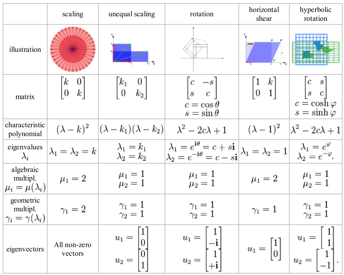
Rotation\begin_inset Separator latexpar\end_inset
⎡⎢⎣ cos(θ) − sin(θ) sin(θ) cos(θ) ⎤⎥⎦

With using of Eigenvectors(A) command in maple I obtain following eigenvalues

⎡⎢⎣ cos(θ) + i⋅sin(θ) cos(θ) − i⋅sin(θ) ⎤⎥⎦

and following eigenvectors

⎡⎢⎣ i − i 1 1 ⎤⎥⎦

Со ротацијата мислам дека сака да каже дека еигенвредностите опишуваат кружница. Зависно од таа вредност ќе го „возат“ еигенвекторот по кружницата.
Scaling

A: = ⎡⎢⎣ k 0 0 k ⎤⎥⎦

2.2 Schrodinger equation

An example of an eigenvalue equation where the transformation T is represented in terms of a differential operator is the time-independent Schrodinger equation in quantum mechanics:

H⋅ψ_E = E⋅ψ_E

where H, the Hamiltonian, is a second-order differential operator and ψ_E the wavefunction, is one of its eigenfunctions corresponding to the eigenvalue E, interpreted as its energy.

Bibliography

[1]