\sloppy
1 Rate Distortion Theory
The description of an arbitrary real number requires an infinite number of bits, so a finite representation of a continuous random variable can never be perfect. How well can we do? To frame the question appropriately, it is necessary to define the goodness of a representation of a source.
This is accomplished by defining a distortion measure which is a measure of distance between the random variable and its representation.
The basic problem in rate distortion theory can then be stated as follows:
Given a source distribution and a distortion measure, what is the minimum expected distortion achievable at particular rate? Or, equivalently, what is the minimum rate distortion required to achieve a particular distortion?
It is simpler to describe X1 and X2 together (at the given distortion for each) than to describe each by itself. Why don’t independent problems have independent solutions? Apparently, rectangular grid points (arising from independent descriptions) do not fill up the space efficiently.
Rate distortion theory can be applied to both discrete and continuous random variables. The zero-error data compression theory of Chapter 5 is and important special case of rate distortion theory applied to a discrete source with zero distortion. We begin by considering the simple problem of representing a single continuous random variable by finite number of bits.
1.1 Quantization
In this section we motivate the elegant theory of rate distortion by showing how complicated it is to solve the quantization problem for a single random variable. Since a continuous random source requires infinite precision to represent exactly, we cannot reproduce it exactly using finite-rate code. The question is then to find the best possible representation for any given data rate.
We first consider the problem of representing a single sample from the source. Let the random variable be represented be X and let the representation of X be denoted as X̂(X). If we are given R bits to represent X, the function X̂ can take 2R values. The problem is to find optimum set of values for X̂ (called the reproduction points or code points) and the regions that are associated with each value X̂.
For exampled, let
X ~ N(0, σ2), and assume a squared-error distortion measure. In this case we wish to find the function
X̂(X) such that
X̂ takes on at most
2R values and minimizes
E(X − X̂(X))2 . If we are given one bit to represent
X , it is clear that the bit should distinguish whether or not
X > 0.
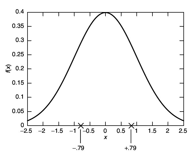
To minimize squared error, each reproduced symbol should be the conditional mean of its region
Претпоставувам условот е да случајната променлива се наоѓа во тој регион.
.
Ова е суштината!!! Изводот од квадратната грешка се пресметува во соодветниот регион.
This is illustrated in
1↓.
Ваквата вредност за X̂ претпоставката е дека ја рачуна со извод од квадратната грешка башка за регионот [0,∞] и башка за регионот [ − ∞, 0]. Подолу претпоставката се покажува како точна!!!
√((2.0)/(π)) = 0.797885
f(x) = (1)/(σ√(2π))⋅e − (x2)/(2⋅σ2)
∫∞ − ∞(x)/(σ⋅√(2π))⋅e − (x2)/(2⋅σ2)dx = ConditionalExpression[0, ℜ(σ2) > 0]
∫∞ − ∞(x2)/(σ⋅√(2π))⋅e − (x2)/(2⋅σ2)dx = ConditionalExpression⎡⎢⎣(1)/(⎛⎝(1)/(σ2)⎞⎠3 ⁄ 2σ), ℜ(σ2) > 0⎤⎥⎦
Assuming⎡⎣σ > 0, ∫∞ − ∞(x2)/(σ⋅√(2π))⋅e − (x2)/(2⋅σ2)dx⎤⎦ = σ2
Assuming⎡⎣σ > 0, ∫∞ − ∞(1)/(σ⋅√(2π))⋅e − (x2)/(2⋅σ2)dx⎤⎦ = 1
(d)/(dx̂)[E(X − X̂)2] = 0 ∫∞ − ∞(x2 − 2⋅x̂⋅x + x̂2)/(σ⋅√(2π))⋅e − (x2)/(2⋅σ2)dx =
∫∞ − ∞(x2)/(σ⋅√(2π))⋅e − (x2)/(2⋅σ2)dx − 2∫∞ − ∞(x⋅x̂)/(σ⋅√(2π))⋅e − (x2)/(2⋅σ2)dx + ∫∞ − ∞(x̂2)/(σ⋅√(2π))⋅e − (x2)/(2⋅σ2)dx = σ2 + x̂2
(d)/(dx̂)(σ2 + x̂2) = 0 → x̂ = 0
——————————————————————————–———————————————————————–
\strikeout off\uuline off\uwave offE + [(X − X̂)2] = ∫∞0(x2)/(σ⋅√(2π))⋅e − (x2)/(2⋅σ2)dx − 2∫∞0(x⋅x̂)/(σ⋅√(2π))⋅e − (x2)/(2⋅σ2)dx + ∫∞0(x̂2)/(σ⋅√(2π))⋅e − (x2)/(2⋅σ2)dx
Assuming⎡⎣σ > 0, ∫∞0(x2)/(σ⋅√(2π))⋅e − (x2)/(2⋅σ2)dx⎤⎦ = (σ2)/(2)
Assuming⎡⎣σ > 0, ∫∞0(x)/(σ⋅√(2π))⋅e − (x2)/(2⋅σ2)dx⎤⎦ = (σ)/(√(2π))
Assuming⎡⎣σ > 0, ∫∞0(1)/(σ⋅√(2π))⋅e − (x2)/(2⋅σ2)dx⎤⎦ = (1)/(2)
(d)/(dx̂)⎛⎝(σ2)/(2) − (2⋅σ)/(√(2π))⋅x̂ + (x̂2)/(2)⎞⎠ = 0 → − σ√((2)/(π)) + x̂ = 0 → \mathchoicex̂ = σ√((2)/(π))x̂ = σ√((2)/(π))x̂ = σ√((2)/(π))x̂ = σ√((2)/(π))
E − [(X − X̂)2] = ∫0 − ∞(x2)/(σ⋅√(2π))⋅e − (x2)/(2⋅σ2)dx − 2∫0 − ∞(x⋅x̂)/(σ⋅√(2π))⋅e − (x2)/(2⋅σ2)dx + ∫0∞(x̂2)/(σ⋅√(2π))⋅e − (x2)/(2⋅σ2)dx
Assuming⎡⎣σ > 0, ∫0 − ∞(x2)/(σ⋅√(2π))⋅e − (x2)/(2⋅σ2)dx⎤⎦ = (σ2)/(2)
Assuming⎡⎣σ > 0, ∫0 − ∞(x)/(σ⋅√(2π))⋅e − (x2)/(2⋅σ2)dx⎤⎦ = − (σ)/(√(2π))
Assuming⎡⎣σ > 0, ∫∞0(1)/(σ⋅√(2π))⋅e − (x2)/(2⋅σ2)dx⎤⎦ = (1)/(2)
(d)/(dx̂)⎛⎝(σ2)/(2) + (2⋅σ)/(√(2π))⋅x̂ + (x̂2)/(2)⎞⎠ = 0 → (2⋅σ)/(√(2π)) + x̂ = 0 → \mathchoicex̂ = − σ√((2)/(π))x̂ = − σ√((2)/(π))x̂ = − σ√((2)/(π))x̂ = − σ√((2)/(π))
Во пресметката на D sе користи изразот за тотална експектација!
D = E[(X − X̂)2] = p(X < 0)⋅E − [(X − X̂)2] + p(X ≥ 0)⋅E + [(X − X̂)2]
= p(X < 0)⋅E − [(X − X̂)2] + p(X ≥ 0)⋅E + [(X − X̂)2] = p(X < 0)⋅E[(X − X̂)2|X < 0] + p(X ≥ 0)⋅E[(X − X̂)2|X ≥ 0] =
(1)/(2)⎛⎝(σ2)/(2) + (2⋅σ)/(√(2π))⋅x̂ + (x̂2)/(2)⎞⎠||x̂ = − σ√((2)/(π)) + (1)/(2)⎛⎝(σ2)/(2) − (2⋅σ)/(√(2π))⋅x̂ + (x̂2)/(2)⎞⎠||x̂ = σ√((2)/(π)) = ⎛⎝(σ2)/(2) − (2⋅σ)/(√(2π))⋅σ√((2)/(π)) + ((σ√((2)/(π)))2)/(2)⎞⎠
⎛⎝(σ2)/(2) − (2⋅σ2)/(π) + (σ2)/(π)⎞⎠ = (σ2)/(2) − (σ2)/(π)
Во Example 1 не се оди со тотална експектација и се добива два пати поголем резултат.
If we are given 2 bits to represent the sample, the situation is not as simple. Clearly we want to divide the real line into four regions and use a point within each region to represent the sample. But it is no longer immediately obvious what the representation regions and the reconstruction points should be. We can, however, state two simple properties of optimal regions and reconstruction points for the quantization of a single random variable:
-
Given a set {X̂(w)} of reconstruction points, the distortion is minimized by mapping a source random variable X to the representation X̂(w) that is closest to it. The set of regions of X defined by these mapping is called a Voronoi or Dirichlet partition defined by the reconstruction points.
-
The reconstruction points should minimize the conditional expected distortion
Овде под кондитионал подразбира conditional expectaton како што и правам во примерот погоре.
over their respective assignment regions.
This two properties enable us to construct a simple algorithm to find a good quantizer: We start with a set of reconstruction points, find the optimal set of reconstruction regions (which are the nearest-neighbor regions with respect to the distortion measure), then find the optimal reconstruction points for these regions (the centroids of these regions if the distortion is squared error), and then repeat the iteration for this new set of reconstruction points. The expected distortion is decreased at each stage in the algorithm, so the algorithm will converge to a local minimum of the distortion. This algorithm is called Lloyd algorithm.
Instead of quantizing a single random variable, let us assume that we are given a set of n i.i.d random variables drawn according to a Gaussian distribution. These random variables are to be represented using nR bits. Since the source is i.i.d, the symbols are independent, and it may appear that the representation of each element is an independent problem to be treated separately. But this is not true, as the results on rate distortion theory will show. We will represent the entire sequence by a single index taking 2nR values. This treatment of entire sequences at once achieves a lower distortion for the same rate than independent quantization of the individual samples.
1.2 Definitions
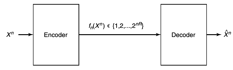
Assume that we have source that produces a sequence
X1, X2, ...Xn i.i.d ~
p(x), x ∈ X. For the proofs in this chapter, we assume that the alphabet is finite, but most of the proofs can be extended to continuous random variables. The encoder describes the source
Xn by an index
fn(Xn) ∈ {1, 2, ..., 2nR}. The decoder represents
Xn by an estimate
X̂n ∈ X̂, as ilustrated in
2↓.
Definition 1: (Distortion Measure)
A distortion function or distortion measure is a mapping
from the set of source alphabet-reproduction alphabet pairs into the set of nonnegative real numbers. The distortion d(x, x̂) is a measure of the cost of representing the symbol x by the symbol x̂.
Definition 2: (Bound of distortion measure)
A distortion measure is said to be bounded if the maximum value of the distortion is finite:
dmax\oversetdef = maxx ∈ X, x̂ ∈ X̂d(x, x̂) < ∞
In most cases, the reproduction alphabet X̂ is the same as the source alphabet X.
Examples of common distortion functions
-
Hamming (probability of error) distortion. The hamming distortion is given by
which results in a probability of error distortion since D = \mathchoiceEd(X, X̂) = Pr(X ≠ X)̂Ed(X, X̂) = Pr(X ≠ X)̂Ed(X, X̂) = Pr(X ≠ X)̂Ed(X, X̂) = Pr(X ≠ X)̂
Овде Ed = E[d] т.е. се работи за експектација.
\strikeout off\uuline off\uwave off
D = Ed(X, X̂) = ∑(x, x̂)p(x, x̂)⋅d(x, x̂) = ∑\overset(x, x̂)x ≠ x̂p(x, x)̂ = P(X ≠ X̂)
-
Squared-error distortion. The squared-error distortion,
is the most popular distortion measure used for continuous alphabets. Its advantages are its simplicity and its relationship to least-squares prediction. But in applications such as image and speech coding, various authors have pointed out that the mean-squared error is not an appropriate measure of distortion for human observers. For example, there is a large squared-error distortion between a speech waveform and another version of the same waveform slightly shifted in time, although both will sound the same to a human observer.
Many alternatives have been proposed; a popular measure of distortion in speech coding is the Itakura-Saito distance, which is the relative entropy between multivariate normal processes. In image coding, however, there is at present no real alternative to using the mean-squared error as the distortion measure.
The distortion measure is defined on a symbol-by-symbol basis. We extend the definition to sequences by using the following definition:
Definition 3: (distortion of blocks of length
n)
The distortion between sequence xn and x̂n is defended by:
So the distortion for a sequence is the average of the per symbol distortion of the elements of the sequence. This is not the only reasonable definition. For example, one may want to measure the distortion between two sequences by the maximum of the per symbol distortions. The theory derived below does not apply directly to this more general distortion measure.
Definition 4 (Distortion - MMV)
А (2nR, n)-rate distortion code consist of an encoding function,
and decoding (reproduction) function,
The distortion associated with the (2nR, n) code is defined as:
where the expectation is with respect to the probability distribution on X:
Веројатно се мисли на Xn!!!
D = ⎲⎳xnp(xn)d(xn, gn(fn(xn)))
The set of
n-tuples
gn(1), gn(2), ..., gn(2nR), denoted by
X̂n(1), ..., X̂n(2nR) constitutes the
codebook, and
f − 1(1), ...f − 1n(2nR) are associated
assignment regions.
Many terms are used to describe the replacement of Xn by its quantized version X̂n(w). It is common to refer to X̂n as the vector quantization, reproduction, reconstruction, representation, source code, or estimate of Xn.
Definition 5 (rate distortion pair):
A rate distortion pair (R, D) is said to be achievable if there exists a sequence of (2nR, n)-rate distortion codes (fn, gn) with limn → ∞Ed(Xn, gn(fn(Xn))) ≤ D.
Definition 6: (rate distortion region):
The rate distortion region for a source is the closure of the set of achievable rate distortion pairs (R, D).
Definition 7: (rate distortion function):
The rate distortion function R(D) is the infinum of rates R such that (R, D) is in the rate distortion region of the source for a given distortion D.
Definition 8: (distortion rate function):
The distortion rate function D(R) is infinum of all distortion D such that (R, D) is in the rate distortion region of the source for a given rate R.
The distortion rate function defines another way of looking at the boundary of the rate distortion region. We will in general use rate distortion function rather than the distortion rate function to describe this boundary, although the two approaches are equivalent.
We now define a mathematical function of the source, which we call the information rate distortion function. The main result of this chapter is the proof that the information rate distortion function is equal to the rate distortion function defined above (i.e. it is the infimum of rates that achieve a particular distortion).
Definition 9: (information rate distortion function)
The information rate distortion function RI(D) for source X with distortion measure d(x, x̂) is defined as:
where the minimization is over all conditional distributions p(x̂|x) for which the joint distribution p(x, x̂) = p(x)p(x̂|x) satisfies the expected distortion constraint.
Paralleling the discussion of channel capacity in Chapter 7, we initially consider the properties of the information rate distortion measures. Late we prove that we can actually achieve this function and calculate it for some simple sources and distortion measures. Later we prove that we can actually achieve this function (i.e., there exist codes with rate R(I)(D) with distortion D). We also prove a converse establishing that R ≥ R(I)(D) for any code that achieves distortion D.
The main theorem of rate distortion theory can now be stated as follows:
Theorem 10.2.1 (Rate Distortion Theorem - MMV)
The rate distortion function for an i.i.d source X with distribution p(x) and bounded distortion function d(x, x̂) is equal to the associated information rate distortion function. Thus,
is the minimum achievable rate at distortion D.
This theorem shows that the operational definition of the rate distortion function is equal to the information definition. Hence we will use R(D) from now on to denote both definitions of the rate distortion function. Before coming to the proof of the theorem, we calculate the information rate distortion function for some simple sources and distortions.
1.3 Calculation of the rate distortion function
1.3.1 Binary Source
We now find the distortion rate R(D) required to describe a Bernoulli(p) source with an expected proportion of errors less than or equal to D.
The rate distortion function for a Bernoulli(p) source with Hamming distortion is given by:
Consider a binary source X ~ Bernoulli(p) with hamming distortion measure. Without loss of generality, we may assume that p < (1)/(2). We wish to calculate the rate distortion function,
R(D) = minp(x̂|x):⎲⎳p(x)p(x̂|x)d(x, x̂) ≤ DI(X;X̂).
Let ⊕ denote modulo 2 addition. Thus, X⊕X̂ = 1 is equivalent to X ≠ X̂.
Многу јака финта!!!
We do not minimize I(X, X̂) directly; instead we find a lower bound and then show that this lower bound is achievable. For any joint distribution satisfying the distortion constraint, we have
I(X;X̂) = H(X) − H(X|X̂) = H(p) − H(X⊕X̂|X̂) ≥ H(p) − H(X⊕X̂) ≥ H(p) − H(D)
\strikeout off\uuline off\uwave off
H(X⊕X̂) = − ∑x = xp(X⊕X̂)⋅log2p(X⊕X̂) = − ∑x = xp(X ≠ X̂)⋅log2p(X ≠ X̂) = H(p(X ≠ X̂))
\mathchoiceD = Ed(X, X̂) = Pr(X ≠ X)̂D = Ed(X, X̂) = Pr(X ≠ X)̂D = Ed(X, X̂) = Pr(X ≠ X)̂D = Ed(X, X̂) = Pr(X ≠ X)̂
since Pr(X ≠ X̂) ≤ D and H(D) increases with D for D ≤ (1)/(2). Thus,
We now show that the lower bound is actually the rate distortion function by finding a joint distribution that meets the distortion constraint and has
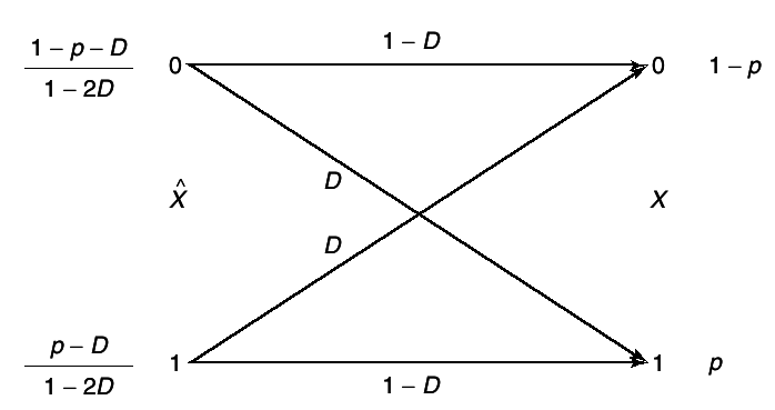
I(X;X̂) = R(D). For
0 ≤ D ≤ p, we can achieve that value of the rate distortion function in
12↑ by choosing
(X, X̂) to have the joint distribution given by the binary symmetric channel shown in
3↓.
We choose the distribution of
X̂ at the input of the channel so that the output distribution of
X is the specified distribution.
Let
r = Pr(X̂ = 1). Then choose
r so that
r(1 − D) + (1 − r)D = p; r − rD + D − rD = p; r(1 − 2D) = p − D;
\mathchoicePr(X̂ = 0) = 1 − r = (1 − 2D − p + D)/(1 − 2D) = (1 − p − D)/(1 − 2D)Pr(X̂ = 0) = 1 − r = (1 − 2D − p + D)/(1 − 2D) = (1 − p − D)/(1 − 2D)Pr(X̂ = 0) = 1 − r = (1 − 2D − p + D)/(1 − 2D) = (1 − p − D)/(1 − 2D)Pr(X̂ = 0) = 1 − r = (1 − 2D − p + D)/(1 − 2D) = (1 − p − D)/(1 − 2D)
If \mathchoiceD ≤ p ≤ (1)/(2)D ≤ p ≤ (1)/(2)D ≤ p ≤ (1)/(2)D ≤ p ≤ (1)/(2), then Pr(X̂ = 1) ≥ 0 and Pr(X̂ = 0) ≥ 0. We then have:
I(X;X̂) = H(X) − H(X|X̂) = H(p) − H(D)
And the expected distortion is Pr(X = X̂) = D.
If
\mathchoiceD ≥ pD ≥ pD ≥ pD ≥ p we can achieve
R(D) = 0 by letting
X̂ = 0 with probability 1. In this case,
I(X, X̂) = 0 and
D = p.
Гледај ја сликата 3↑
Similarly, if
D ≥ 1 − p, we can achieve
R(D) = 0 by setting
X̂ = 1 with probability
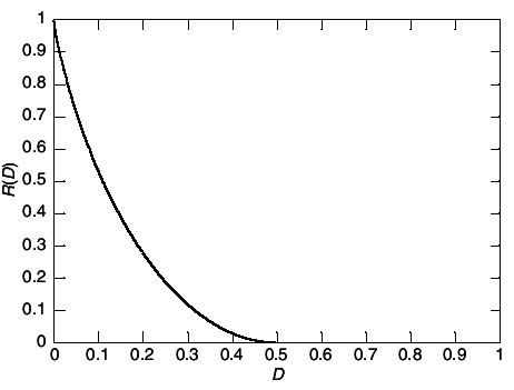
1. Hence rate distortion function for a binary source is:
Ова го имам имплементирано во Maple.
This function is illustrated
The above calculations may seem entirely unmotivated. Why should minimizing mutual information have anything to do with quantization?
The answer to this question must wait until we prove Theorem 10.2.1.
1.3.2 Gaussian Source
Although Theorem 10.2.1 is proved only for discrete sources with bounded distortion measure, it can also be proved for well-behaved continuous sources and unbounded distortion measures. Assuming this general theorem, we calculate the rate distortion function for a Gaussian source with squared-error distortion.
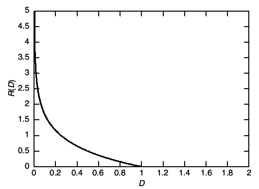
The rate distortion function for a N(0, σ2) source with squared-error distortion is
Let X be ~N(0, σ2). By the rate distortion theorem extended to continuous alphabets, we have:
As in the preceding example, we first find a lower bound for the rate distortion function and then prove that this is achievable. Since E(X − X̂)2 ≤ D , we observe that
I(X;X̂) = h(X) − h(X|X̂) = (1)/(2)log(2πe)σ2 − h(X − X̂|X̂)\overset(a) ≥ (1)/(2)log(2πe)σ2 − h(X − X̂) ≥
\overset(b) ≥ (1)/(2)log(2πe)σ2 − h(N(0, E(X − X̂)2)) =
= (1)/(2)log(2πe)σ2 − (1)/(2)log(2πe)E(X − X̂)2 ≥ (1)/(2)log(2πe)σ2 − (1)/(2)log(2πe)D = (1)/(2)log⎛⎝(σ2)/(D)⎞⎠
where (a) follows for the fact that conditioning reduces entropy and (b) follows form the fact that the normal distribution maximize the entropy for a given second moment (Theorem 8.6.5). Hence,
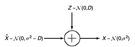
To find the conditional density
f(x̂|x) that achieves this lower bound, it is usually more convenient to look at the conditional density
f(x|x̂) , which is sometimes called the
test channel (thus emphasizing the duality of rate distortion with channel capacity). As in the binary case, we construct
f(x|x̂) to achieve equality in the bound. We choose the joint distribution as shown in
5↑. If
D ≤ σ2, we chose
where X̂ are independent
σ̂2 = σ2 − D
. For this joint distribution, we calculate
and
E(X − X̂)2 = D, thus achieving the bound in
17↑. If
D ≥ σ2, we choose
X̂ = 0 with probability 1, achieving
R(D) = 0. Hence, the rate distortion function for the Gaussian source with squared-error distortion is:
Оваа слика и претходната ги добив во мапле врз основ на изразите
20↑ 8↑. Во 2D plot се добиваат за фикни вредносит на
p (како контурен plot). Направив и 3D плотови, но поентата е иста.
We can rewrite
20↑ to express the distortion in terms of the rate,
\mathchoiceD(R) = σ22 − 2RD(R) = σ22 − 2RD(R) = σ22 − 2RD(R) = σ22 − 2R
log(σ2)/(D) = 2⋅R; σ2 = D⋅22R; D = σ22 − 2R;
Each additional bit of description reduces the expected distortion by a factor of 4.
Тука ми текна дека изразот за rate distortion функцијата за бинарен канал R(D) = H(p) − H(D). Сака да каже дека ако нема дисторзија тогаш изворот можеш да го опишеш со H(p) бити, нормално ако прифатиш да има одредена дисторзија изворот можеш да го опишеш со помал број на бити.
With a 1-bit description, the best expected square error is
(σ2)/(4) = 0.25σ2. We can compare this with the result of simple 1-bit quantization of a
N(0, σ2) random variable as described in Section 10.1. In this case, using the two regions corresponding to the positive and negative real lines and reproduction points as the centroids of the respective regions, the expected distortion is
((π − 2))/(π)⋅σ2 = 0.3633⋅σ2
(See Problem 10.1) i.e. Box below!
. As we prove later, the rate distortion limit
R(D) is achieved by considering long block lengths. This example shows that we can achieve a lower distortion by considering several distortion problems in succession (long block lengths) that can be achieved by considering each problem separately. This is somewhat surprising because we are quantizing independent random variables.
\mathchoicex̂1, 2 = ±σ√((2)/(π))x̂1, 2 = ±σ√((2)/(π))x̂1, 2 = ±σ√((2)/(π))x̂1, 2 = ±σ√((2)/(π))
D = E[(X − X̂)2] = ∫0 − ∞((x − x1̂)2)/(σ⋅√(2π))⋅e − (x2)/(2⋅σ2)dx + ∫∞0((x − x2̂)2)/(σ⋅√(2π))⋅e − (x2)/(2⋅σ2)dx
\strikeout off\uuline off\uwave offAssuming⎡⎣σ > 0, ∫0 − ∞((x + σ⋅√((2)/(π)))2)/(σ⋅√(2π))⋅e − (x2)/(2⋅σ2)dx⎤⎦ = ((π − 2)σ2)/(2π)
Assuming⎡⎣σ > 0, ∫∞0((x − σ⋅√((2)/(π)))2)/(σ⋅√(2π))⋅e − (x2)/(2⋅σ2)dx⎤⎦ = ((π − 2)σ2)/(2π)
D = 2⋅((π − 2)σ2)/(2π) = ((π − 2)σ2)/(π) = σ2 − (2σ2)/(π)
Да ова е вака ако не одиш со тотална експектација како што одам во Example 1!!!?
Таму добив:
⎛⎝(σ2)/(2) − (2⋅σ2)/(π) + (σ2)/(π)⎞⎠ = (σ2)/(2) − (σ2)/(π)
два пати е помало зошто множам со веројатностите да променливите се најдат во соодветниот регион.
1.3.3 Simultaneous Description of Independent Gaussian Random Variables
Consider the case of representing m independent (but not identically distributed) normal random sources X1, ..., Xm, where Xi are ~ N(0, σ2i), with squared-error distortion. Assume that we are given R bits with which to represent this random vector. The question naturally arises as to how we should allot these bits to the various components to minimize the total distortion.
Тука ми текна на примерот од глава 15 со температурата на двата града (Gotham и Metropolis). Температурата (сончево, облачно) ја праќа со еден бит.
Extending the definition of the information rate distortion function to the vector case, we have
R(D) = minf(x̂m|xm):Ed(Xm, X̂m) ≤ DI(Xm;X̂m)
where \mathchoiced(xm, x̂m) = ∑mi = 1(xi − x̂i)2d(xm, x̂m) = ∑mi = 1(xi − x̂i)2d(xm, x̂m) = ∑mi = 1(xi − x̂i)2d(xm, x̂m) = ∑mi = 1(xi − x̂i)2. Now using the arguments in the preceding example, we have
I(Xm;X̂m) = h(Xm) − h(Xm|X̂m) = ∑mi = 1h(Xi) − ∑mi = 1h(Xi|Xi − 11, X̂m) = ∑mi = 1h(Xi) − ∑mi = 1h(Xi|X̂m)\overset(a) ≥ ∑mi = 1h(Xi) − ∑mi = 1h(Xi|Xî)
= ∑mi = 1I(Xi;X̂i)\overset(b) ≥ ∑mi = 1R(Di) = ∑mi = 1⎛⎝(1)/(2)⋅log(σ2i)/(Di)⎞⎠\mathchoice + + + +
where Di = E(Xi − Xî)2 and (a) follows form the fact that conditioning reduces entropy. We can achieve equality in (a) by choosing f(xm|x̂m) = ∏mi = 1f(xi|x̂i) and in (b) by choosing the distribution of each \mathchoiceX̂i ~ N(0, σ2i − Di)X̂i ~ N(0, σ2i − Di)X̂i ~ N(0, σ2i − Di)X̂i ~ N(0, σ2i − Di) as in the preceding example. Hence the problem of finding the rate distortion function can be reduced to the following optimization (using nats for convenience):
\strikeout off\uuline off\uwave off
Ed(Xm, X̂m) = ⎲⎳(xm, x̂m)p(xm, x̂m)d(xm, x̂m) = ||d(xm, x̂m) = (1)/(m)m⎲⎳i = 1d(xi, x̂i)|| = (1)/(m)⋅ ⎲⎳(xm, x̂m)p(xm, x̂m)⋅m⎲⎳i = 1d(xi, x̂i) =
= (1)/(m)⋅m∏j = 1p(xj, xĵ)⋅m⎲⎳i = 1d(xi, x̂i) = m⎲⎳i = 1p(xi, x̂i)d(xi, x̂i) = ⎲⎳iDi ≤ D
Многу ова е диво! Треба со пример од
m = 2 да се провери како излегуваат сумите и производите.
Всушност дефинитивно треба со квадратна дисторзија на грешка (squared error distortion).
\strikeout off\uuline off\uwave off
d(xm, x̂m) = m⎲⎳i = 1(xi − x̂i)2
\strikeout off\uuline off\uwave off
Ed(Xm, X̂m) = ⎲⎳(xm, x̂m)p(xm, x̂m)⋅d(xm, x̂m) =
= m⎲⎳i = 1p(xi, xî)⋅(xi − x̂i)2 = ⎲⎳iDi ≤ D
Using Lagrange multipliers, we construct the functional
and differentiating with respect to Di and setting equal to 0, we have
Hence, the optimum allotment of the bits to the various descriptions results in an equal distortion for each variable. This is possible if the constant
λ’ increases until it exceeds
σ2i for some
i. At this point the solution
24↑ is on the boundary of the allowable region of distortions. If we increase the total distortion, we must use the Kuhn-Tucker conditions to find the minimum in
22↑. In this case the Kuhn-Tucker conditions yield
(∂J)/(∂Di) = − (1)/(2)⋅(1)/(Di) + λ
where λ is chosen so that:
(∂J)/(∂Di)⎧⎨⎩
= 0
if Di < σ2i
≤ 0
if Di ≥ σ2i
It is easy to check that the solution to the Kuhn-Tucker equations is given by the following theorem:
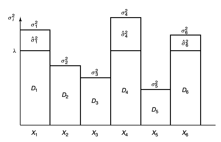
Theorem 10.3.3 (Rate distortion for a parallel Gaussian source)
Let Xi = N(0, σ2i), i = 1, 2, ..., m be independent Gaussian random variables, and let the distortion measure be \strikeout off\uuline off\uwave off\mathchoiced(xm, x̂m) = ∑mi = 1(xi − x̂i)2d(xm, x̂m) = ∑mi = 1(xi − x̂i)2d(xm, x̂m) = ∑mi = 1(xi − x̂i)2d(xm, x̂m) = ∑mi = 1(xi − x̂i)2.
\strikeout off\uuline off\uwave offЗошто не го дели со m? Се коси со Eq10.6.
Then the rate distortion function is given by:
where
Di = ⎧⎨⎩
λ
if λ < σ2i
σ2
ifλ ≥ σ2i
where λ is chosen so that \mathchoice∑mi = 1Di = D∑mi = 1Di = D∑mi = 1Di = D∑mi = 1Di = D.
This gives rise to a kind of reverse water-filling, as illustrated in
7↑.
Види 18↑ σ̂2 = σ2 − D
We choose a constant
λ and only describe those random variables with variances greater that
λ.
No bits are used to describe random variables with variance less than λ.
Ова е вака затоа што σ̂2 = σ2i − Di = 0 практично не постои таа репродукција.
Summarizing, if
X ~ N⎛⎜⎜⎜⎝0, ⎡⎢⎢⎢⎣
σ21
...
0
...
...
...
0
...
σ2m
⎤⎥⎥⎥⎦⎞⎟⎟⎟⎠, then X̂ ~ N⎛⎜⎜⎜⎝0, ⎡⎢⎢⎢⎣
σ̂21
...
0
...
...
...
0
...
σ̂2m
⎤⎥⎥⎥⎦⎞⎟⎟⎟⎠
and E(Xi − X̂i)2 = Di where \mathchoiceDi = min{λ, σ2i}Di = min{λ, σ2i}Di = min{λ, σ2i}Di = min{λ, σ2i}.
\strikeout off\uuline off\uwave offX̂i ~ N(0, σ2i − Di)
More generally, the rate distortion function for a multivariate normal vector can be obtained by reverse water-filling on the eigenvalues. We can also apply the same arguments to a Gaussian stochastic process. By the spectral representation theorem, a Gaussian stochastic process can be represented as an integral of independent Gaussian processes in the various frequency bands. Reverse water-filling on the spectrum yields the rate distortion function
Ова не баш го контам!!!
.
1.4 Converse to the rate distortion theorem
In this section we prove the converse of Theorem 10.2.1 by showing that we cannot achieve a distortion of less than D if we describe X at rate less than R(D), where
The minimization is over all conditional distributions
p(x̂|x) for which the joint distribution
p(x, x̂) = p(x)p(x̂|x) satisfies expected distortion constraint. Before proving the converse, we establish some simple properties of the information rate distortion function.
Lemma 10.4.1 ( Convexity of
R(D))
The rate distortion function
R(D) given in
26↑ is a non-increasing convex function of
D.
R(D) is the minimum of the mutual information over increasingly larger sets as D increases. Thus, R(D) is non-increasing in D. То prove thatR(D) is convex, consider two rate distortion pairs, (R1, D1) and (R2, D2), which lie on the rate distortion curve. Let the joint distributions that achieve these pairs be p1(x, x̂) = p(x)p1(x̂|x) and p2(x, x̂) = p(x)p2(x̂|x). Consider the distribution pλ = λp1 + (1 − λ)p2. Since the distortion is a linear function of the distribution, we have D(pλ) = λD1 + (1 − λ)D2 . Mutual information, on the other hand, is a convex function of the conditional distribution (Theorem 2.7.4), and hence
Hence, by the definition of the rate distortion function
R(Dλ) ≤ Ipλ(X, X̂) ≤ λIp1(X;X̂) + (1 − λ)Ip2(X;X̂) = λR(D1) + (1 − λ)R(D2)
which proves that R(D) is convex function of D.
The converse can now be proved.
Proof: (Converse in Theorem 10.2.1)
We must show for any source X drawn i.i.d. ~ p(x) with distortion measure d(x, x̂) and any (2nR, n) rate distortion code with distortion ≤ D , that the rate R of the code satisfies R ≥ R(D). In fact, we prove that R ≥ R(D) even for randomized mappings fn and gn, as long as fn takes on at most 2nR values.
Consider any
(2nR, n) rate distortion code defined by functions
fn and
gn as given in
6↑
\strikeout off\uuline off\uwave offfn:Xn → {1, 2, ...2nR}
an
7↑
g:{1, 2, ..., 2nR} → X̂n
. Let
X̂n = X̂n(Xn) = gn(fn(Xn)) be the reproduced sequence corresponding to
Xn. Assume that
Ed(Xn, X̂n) ≥ D for this code. Then we have the following chain of inequalities:
\mathchoicenRnRnRnR\overset(a) ≥ H(fn(Xn))\overset(b) ≥ H(fn(Xn)) − H(fn(Xn)|Xn) = I(Xn;fn(Xn))\overset(c) ≥ I(Xn;X̂n) =
= H(Xn) − H(Xn|X̂n)\overset(d) = n⎲⎳i = 1H(Xi) − H(Xn|X̂n)\overset(e) =
= n⎲⎳i = 1H(Xi) − n⎲⎳i = 1H(Xi|X̂nXi − 1, ..., X1)\overset(f) ≥ n⎲⎳i = 1H(Xi) − n⎲⎳i = 1H(Xi|X̂i) =
= \mathchoicen⎲⎳i = 1I(Xi;X̂i)\overset(g) ≥ n⎲⎳i = 1R(Ed(Xi, X̂i))n⎲⎳i = 1I(Xi;X̂i)\overset(g) ≥ n⎲⎳i = 1R(Ed(Xi, X̂i))n⎲⎳i = 1I(Xi;X̂i)\overset(g) ≥ n⎲⎳i = 1R(Ed(Xi, X̂i))n⎲⎳i = 1I(Xi;X̂i)\overset(g) ≥ n⎲⎳i = 1R(Ed(Xi, X̂i)) = n⎛⎝(1)/(n)n⎲⎳i = 1R(Ed(Xi, X̂i))⎞⎠\overset(h) ≥
n⋅R⎛⎝(1)/(n)⋅n⎲⎳i = 1Ed(Xi, X̂i)⎞⎠\overset(i) = nR(Ed(Xn, X̂n))\overset(j) = \mathchoicenR(D)nR(D)nR(D)nR(D)
(a) follows from the fact that the range of fn is at most 2nR
(b) follows form the fact that H(fn(Xn)|Xn) ≥ 0
(c) follows from the data processing inequality
(d) follows from the fact that Xi are independent
(e) follows from the chain rule for entropy
(f) follows from the fact that conditioning reduces entropy
(g) follows form the definition of rate distortion function
(h) follows from the convexity of the rate distortion function (Lemma 10.4.1) and Jensen’s inequality
(i) follows from the definition of distortion for blocks of length
n (
5↑)
(j) follows form the fact that R(D)is non-increasing function of D and Ed(Xn, X̂n) ≤ D
Ова е земено како претпоставка во теоремата!
.
Многу сличен доказ има за Rate Distortion with side information Глава 15.9
This shows that the rate R of any rate distortion code exceeds the rate distortion function R(D) evaluated at the distortion level D = Ed(Xn, X̂n) achieved by that code.
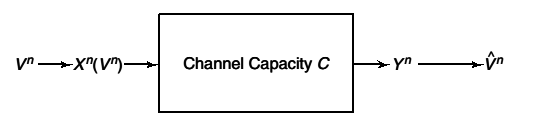
A similar argument can be applied when the encoded source is passed through a noisy channel and hence we have the equivalent of the source channel separation theorem with distortion:
Theorem 10.4.1 (Source-channel separation theorem with distortion)
Let V1, V2, ..., Vn be finite alphabet i.i.d source which is encoded as a sequence of n input symbols Xn of a discrete memory-less channel with capacity C. The output of the channel Yn is mapped onto the reconstruction alphabet V̂n = g(Yn). Let D = Ed(Vn, V̂n) = (1)/(n)∑ni = 1Ed(Vi, V̂i) be the average distortion achieved by this combined source and channel coding scheme. Then the distortion D is achievable only if \mathchoiceC ≥ R(D)C ≥ R(D)C ≥ R(D)C ≥ R(D).
Сака да каже дека ако пренесуваш без дисторзија тогаш C ≥ H(X), а ако дозволуваш дисторзија тогаш C ≥ R(D)
.
Proof: See problem 10.17
1.5 Achievability of the rate distortion function
We now prove the achievability of the rate distortion function. We begin with a modified version of the joint AEP in which we add the condition that the pair of sequences be typical with respect to the distortion measure.
Let p(x, x̂) be a joint probability distortion of XxX̂ and let d(x, x̂) be a distortion measure on XxX̂. For any ϵ > 0 , a pair of sequences (xn, x̂n) is said to be distortion ϵ-typical or simply distortion typical if
\mathchoice|| − (1)/(n)logp(xn) − H(X)|| < ϵ; || − (1)/(n)logp(x̂n) − H(X̂)|| < ϵ; || − (1)/(n)logp(xn, x̂n) − H(X, X̂)|| < ϵ; |d(xn, x̂n) − Ed(X, X̂)| < ϵ|| − (1)/(n)logp(xn) − H(X)|| < ϵ; || − (1)/(n)logp(x̂n) − H(X̂)|| < ϵ; || − (1)/(n)logp(xn, x̂n) − H(X, X̂)|| < ϵ; |d(xn, x̂n) − Ed(X, X̂)| < ϵ|| − (1)/(n)logp(xn) − H(X)|| < ϵ; || − (1)/(n)logp(x̂n) − H(X̂)|| < ϵ; || − (1)/(n)logp(xn, x̂n) − H(X, X̂)|| < ϵ; |d(xn, x̂n) − Ed(X, X̂)| < ϵ|| − (1)/(n)logp(xn) − H(X)|| < ϵ; || − (1)/(n)logp(x̂n) − H(X̂)|| < ϵ; || − (1)/(n)logp(xn, x̂n) − H(X, X̂)|| < ϵ; |d(xn, x̂n) − Ed(X, X̂)| < ϵ
The set of distortion typical sequences is called the distortion typical set and is denoted A(n)d, ϵ .
Note that this is the definition of the jointly typical set (Section 7.6) with the additional constraint that the distortion e close to the expected value. Hence the distortion typical set is subset of the jointly typical set (i.e. \mathchoiceA(n)d, ϵ ⊂ A(n)ϵA(n)d, ϵ ⊂ A(n)ϵA(n)d, ϵ ⊂ A(n)ϵA(n)d, ϵ ⊂ A(n)ϵ). If (Xi, X̂i) are drawn i.i.d ~p(x, x̂), the distortion between two random sequences
d(Xn, X̂n) = (1)/(n)⋅n⎲⎳i = 1d(Xi, X̂i)
is an average of i.i.d random variables, and the law of large numbers implies that it is close to its expected value with high probability. Hence we have the following lemma.
Let (Xi, X̂i) be drawn i.i.d ~p(x, x̂). Then Pr((Xi, X̂i) ∈ A(n)d, ϵ) → 1 as n → ∞.
The sums in the four conditions in the definition of A(n)d, ϵ are all normalized sums of i.i.d random variables and hence, by the law of large numbers tend to their respective expected values with probability 1. Hence the set of sequences satisfying all four conditions has probability tending to 1 as n → ∞.
The following lemma is direct consequence of the definition of the distortion typical set.
For all (xn, x̂n) ∈ A(n)d, ϵ;
Using the definition of A(n)d, ϵ we can bound the probabilities p(xn), p(x̂n) and p(xn, x̂n) for all (xn, x̂n) ∈ A(n)d, ϵ and hence
\mathchoicep(x̂n|xn)p(x̂n|xn)p(x̂n|xn)p(x̂n|xn) = (p(xn, x̂n))/(p(xn)) = p(x̂n)⋅(p(xn, x̂n))/(p(xn)p(x̂n)) ≤ p(x̂n)⋅(2 − n(H(X, X̂) − ϵ))/(2 − n(H(X) + ϵ)⋅2 − n(H(X̂) + ϵ)) = 2 − n(H(X, X̂) − ϵ)⋅2 − n( − H(X) − ϵ)⋅2 − n( − H(X̂) − ϵ)
≤ p(x̂n)⋅2 − n(H(X, X̂) − 3ϵ − H(X) − H(X̂)) =
H(X, X̂) = H(X̂) + H(X|X̂); H(X, X̂) − H(X̂) = H(X|X̂)
= p(x̂n)⋅2 − n(H(X|X̂) − 3ϵ − H(X)) = p(x̂n)⋅2 − n( − I(X;X̂) − 3ϵ) = \mathchoicep(x̂n)⋅2n(I(X;X̂) + 3ϵ)p(x̂n)⋅2n(I(X;X̂) + 3ϵ)p(x̂n)⋅2n(I(X;X̂) + 3ϵ)p(x̂n)⋅2n(I(X;X̂) + 3ϵ)
and the Lemma follows immediately.
We also need the following interesting inequality.
Lemma 10.5.3 (Многу корисна математичка нееднаквост)
For 0 ≤ x, y ≤ 1, n > 0
Let f(y) = e − y − 1 + y. Then f(0) = 0 and f’(y) = − e − y + 1 > 0 for y > 0, and hence f(y) > 0 for y > 0. Hence for 0 ≤ y ≤ 1 we have e − y ≥ 1 − y , and racing this to the n-th power , we obtain
(1 − y)n ≤ e − yn
e − 0.01 = 0.99004983374917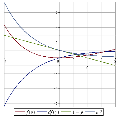 f(y) > 0; e − y − 1 + y > 0; e − y ≥ 1 − y
Thus the lemma is satisfied for x = 1. By examination, it is clear that the inequality is also satisfied for x = 0. By differentiation, it is easy to see that gy(x) = (1 − xy)n is convex function of x , and hence for 0 ≤ x ≤ 1, we have
(1 − xy)n = gy(x)\overset(a) ≤ (1 − x)gy(0) + x⋅gy(1) = (1 − x)1n + x⋅(1 − y)n ≤ (1 − x) + x⋅e − yn ≤ 1 − x + e − yn
(a) Ова следи од дефиницијата на конвексна функција
gy(x) = gy(x⋅1 + (1 − x)⋅0) = x⋅gy(1) + (1 − x)⋅gy(0)
We use the preceding proof to prove the achievability of Theorem 10.2.1
Proof: (Achievability in Theorem 10.2.1)
Let
X1, X2, ..., Xn be drawn i.i.d. ~
p(x) and let
d(x, x̂) be a bounded distortion measure for this source. Let the rate distortion function for this source be
R(D). Then for any
D, and any
R > R(D), we will show that rate distortion pair
(R, D) by proving the existence of sequence of rate distortion codes with rate
R and asymptotic distortion
D. Fix
p(x̂|x) where
p(x̂|x) achieves equality in
26↑
R(D) = minp(x̂|x):∑(x, x̂)p(x)p(x̂|x)d(x, x̂) ≤ DI(X;X̂)
. Thus,
I(X;X̂) = R(D). Calculate
p(x̂) = ∑xp(x)p(x̂|x). Chose
δ > 0. We will prove the existence of a
rate distortion code with rate
R and distortion less than or equal to
D + δ.
Randomly generate a rate distortion code-book C consisting of 2nR sequences X̂n drawn i.i.d ~∏ni = 1p(x̂i). Index these codewords by w ∈ {1, 2, ..., 2nR}. Reveal this code-book to the encoder and decoder.
Encode Xn by w if there exists a w such that (Xn, X̂n(w)) ∈ A(n)d, ϵ, the distortion typical set. If there is more then one such w, send the least. If there is no such w, let w = 1 . Thus, nR bits suffice to describe the index w of the joint typical codeword.
The reproduced sequence is X̂n(w).
Calculation of distortion:
As in the case of the channel coding theorem, we calculate the expected distortion over the random choice of codebooks C as:
where the expectation is over the random choice of codebooks and over Xn.
For fixed codebook C and choice of ϵ > 0, we divide the sequences xn ∈ Xn into two categories:
-
Sequences xn such that there exists a codeword X̂n that is distortion typical with xn [i.e., d(xn, x̂n) < D + ϵ]. Since the total probability of these sequences is at most 1, these sequences contribute at most D + ϵ to the expected distortion.
-
Sequences xn such that there does not exist a codeword X̂n(w) that is distortion typical with xn. Let Pe be total probability of these sequences. Since the distortion for any individual sequence is bounded by dmax, these sequences contribute at most Pedmax to the expected distortion.
Hence, we can bound the total distortion by
which can be made less than D + δ for an appropriate choice of ϵ if Pe is small enough. Hence, if we show that Pe is small, then expected distortion is close to D and the theorem is proved.
We must bound the probability that for a random choice of code-book C and randomly chosen source sequence, there is no codeword that is distortion typical with the source sequence. Let J(C) denote the set of source sequences xn such that at least one codeword in C is distortion typical with xn. Then
this is the probability of all sequences not well represented by a code, averaged over the randomly chosen code. By changing the order of summation we can also interpret this as the probability of choosing a codebook that does not well represent sequence xn, averaged to respect to p(xn). Thus,
The probability that a single randomly chosen codeword X̂n does not well represent a fixed xn is
and therefore the probability that 2nR independently chosen codewords do not represent xn, averaged over p(xn), is
Pe = ⎲⎳xnp(xn)[1 − ⎲⎳x̂np(x̂n)K(xn, x̂n)]nR
We now use Lemma 10.5.2
p(x̂n) ≥ p(x̂n|xn)⋅2 − n(I(X;X̂) + 3ϵ)
to bound the sum within the brackets. From Lemma 10.5.2, it follows that
⎲⎳x̂np(x̂n)K(xn, x̂n) ≥ ⎲⎳x̂np(x̂n|xn)⋅2 − n(I(X;X̂) + 3ϵ)K(xn, x̂n)
and hence
We now use Lema 10.5.3
(1 − xy)n ≤ 1 − x + e − yn.
to bound the term on the right side of
36↑ and obtain
substituting this inequality in
36↑ we obtain
Pe ≤ ⎲⎳xnp(xn)(1 − ⎲⎳x̂np(x̂n|xn)⋅K(xn, x̂n) + e − 2 − n(I(X;X̂) + 3ϵ)⋅2nR) =
The last term in the bound is equal to:
e − 2 − n(I(X;X̂) + 3ϵ)⋅2nR = e − 2n(R − I(X;X̂) − 3ϵ)
which goes to zero exponentially high with
n if
\mathchoiceR > I(X;X̂) + 3ϵR > I(X;X̂) + 3ϵR > I(X;X̂) + 3ϵR > I(X;X̂) + 3ϵ . H
ence if we choose p(x̂|x) to be the conditional distribution that achieves the minimum in the rate distribution function, then
R > R(D) implies that
R > I(X;X̂) and we can chose
ϵ small enough so that the last term in
38↑ goes to
0.
Tis first two terms in
38↑ give the probability under the joint distribution
p(xn, x̂n) that the pair of sequences is not distortion typical. Hence, using Lemma 10.5.1, we obtain
Pϵ = 1 − ⎲⎳xn ⎲⎳x̂np(xnx̂n)⋅K(xn, x̂n) = Pr((Xn, X̂n)∉And, ϵ) ≤ ϵ
for n sufficiently large. Therefore, by an appropriate choice of ϵ and n, we can make Pe as small as we like.
So, for any choice of δ > 0, there exists an ϵ and n such that over all randomly chosen rate R codes of block length n, the expected distortion is less than D + δ. Hence, there must exist at least one code C* with this rate and block length with average distortion less than D + δ. Since δ was arbitrary, we have shown that (R, D) is achievable if R > R(D).
We have proved the existence of a rate distortion code with an expected distortion close to D and rate close to R(D). The similarities between the random coding
proof of the rate distortion theorem and the random coding proof of the channel coding theorem are now evident. We will explore the parallels further by considering the Gaussian example, which provides some geometric insight into the problem. It turns out that channel coding is sphere packing and rate distortion coding is sphere covering.
Channel coding for the Gaussian channel (MMV).
Consider a Gaussian channel, Yi = Xi + Zi where Zi are i.i.d. ~ N(0, N) and there is a power constraint P on the power per symbol of the transmitted codeword. Consider the sequence of n transmissions. The power constraint implies that the transmitted sequence lies within a sphere of radius √(nP) in ℛn. The coding problems is equivalent to finding a set of 2nR sequences within this sphere such that the probability of any of them being mistaken for any other is small - the spheres of radius √(nN) around each of them are almost disjoint. This corresponds to filling a sphere of radius √(n(P + N)) with spheres of radius √(nN). One would expect that the largest number of spheres that could be fit would be the ratio of the volumes, or, equivalently, the n-th power of the ratio of their radii. Thus, if M is the number of codewords that can be transmitted efficiently, we have
the results of the channel coding theorem show that it is possible to do this efficiently for large n; it is possible to find approximately
2nC ≥ M; nC ≥ log2(M); C ≥ (1)/(n)log2(M)
R = (1)/(n)logM ≤ C → M ≤ 2nC Затоа во
39↑ го става овој израз и го добива
40↑.
Ако удриш логаритам лево и десно во
40↑ ќе добиеш:
nC = (n)/(2)log2⎛⎝1 + (P)/(N)⎞⎠ → C = (1)/(2)log2⎛⎝1 + (P)/(N)⎞⎠
codewords such that the noise spheres around them are almost disjoint (the total volume of their intersection is arbitrarily small).
Многу е јака геометрискава интерпретација. Од неа (види Box) практично ја добиваш формулата за капацитет на гаусов канал. Истава интерпретација ја има и во Глава 9 EIT.
Rate distortion for the Gaussian source.
Consider the Gaussian source of variance σ2. A (2nR, n) rate distortion code for this source with distortion D is set of 2nR sequences in ℛn such that most source sequences of length n (all those that lie within a sphere of radius √(nσ2) ) are within a distance √(nD) of some codeword. Again, by the sphere-packing argument, it is clear that the minimum number of codewords required is:
The rate distortion theorem shows that this minimum rate is asymptotically achievable (i.e., that there exists, a collection of spheres of radius √(nD) that cover the space except for a set of arbitrarily small probability).
The above geometric arguments also enable us to transform a good code for channel transmission into a good code for rate distortion. In both cases, the essential idea is to fill the space of source sequences: In channel transmission, we want to find the largest set of codewords that have a large minimum distance between codewords, whereas in rate distortion, we wish to find the smallest set of codewords that covers the entire space. If we have any set that meets the sphere packing bound for one, it will meet sphere packing bound for the other. In the Gaussian case, choosing the codewords to be Gaussian with the appropriate variance is asymptotically optimal for both rate distortion and channel coding.
1.6 Strongly typical sequences and rate distortion
In Section 10.5 we proved the existence of a rate distortion code of rate
R(D) with
average distortion close to D. In fact, not only is the average distortion close to
D, but the total probability that the distortion is greater than
D + δ is close to
0. The proof of this is similar to the proof in Section 10.5; the main difference is that we will use strongly typical sequences rather than weakly typical sequences. This will enable us to give an upper bound to the probability that a typical source sequence is not well represented by a randomly chosen codeword in
35↑
Pr((xn, X̂n)∉And, ϵ) = Pr(K(xn, X̂n) = 0) = 1 − ∑x̂np(x̂n)K(xn, x̂n)
. We now outline the alternative proof based on strong typicality that will provide a stronger and more intuitive approach to the rate distortion theorem.
We begin by defining strong typicality and quoting a basic theorem bounding the probability that two sequences are jointly typical. The properties of strong typicality were introduced by Berger
[1] and were explored in detail in the book by Csiszar and Korner
[2]. We will define strong typicality (as in Chapter 11) and state a
fundamental lemma (Lemma 10.6.2).
Definition (strong typicality)
As sequence xn ∈ Xn is said to be ϵ-strongly typical with respect to a distribution p(x) on X if:
1. For all a ∈ X with p(a) > 0, we have
2. Fora all a ∈ X with p(a) = 0, N(a|xn) = 0.
N(a|xn) is the number of occurrences of symbol a in the sequence xn.
The set of sequences xn ∈ Xn such that xn is strongly typical is called the strongly typical set and is denoted A*(n)ϵ(X) or A*(n)ϵ when the random variable is understood from the context.
Definition (joint strong typicality)
A pair of sequences (xn, yn) ∈ XnxYn is said to be ϵ-strongly typical with respect to distribution p(x, y) on XxY if:
1. For all (a, b) ∈ XxY with p(a, b) > 0, we have
2. For all (a, b) ∈ XxY with p(a, b) = 0, N(a, b|xn, yn) = 0.
N(a, b|xn, yn) is the number of occurrences of the pair (a, b) in the pair of sequences (xn, yn).
The set of sequences (xn, yn) ∈ XnxYn such as (xn, yn) is strongly typical is called the strong-typical set and is denoted A*(n)ϵ(X, Y) or A*(n)ϵ. From the definition, it follows that if (xn, yn) ∈ A*(n)ϵ(X, Y) then xn ∈ A*(n)ϵ(X) . From strong law of large numbers, the following lemma is immediate.
Let (Xi, Yi) be drawn i.i.d. ~p(x, y) . Then Pr((Xi, Yi) ∈ A*(n)ϵ) → 1 as n → ∞
We will use one basic result, which bounds the probability that an independently drawn sequence will be seen as jointly strongly typical with a given sequence. Theorem 7.6.1 shows that if we chose Xn and Yn independently the probability that they will be weekly jointly typical is \thickapprox2 − nI(X;Y). The following lemma extends the result to strongly typical sequences. This is stronger that the earlier result in that it gives a lower bound on the probability that a randomly chosen sequence is jointly typical with a fixed typical xn.
Let Y1, Y2, ..., Yn be drawn i.i.d., ~ p(y). For xn ∈ A*(n)ϵ(X), the probability that (xn, Yn) ∈ A*(n)ϵ is bounded by:
\mathchoice2 − n(I(X, Y) + ϵ1) ≤ Pr((xn, Yn) ∈ A*(n)ϵ) ≤ 2 − n(I(X, Y) − ϵ1)2 − n(I(X, Y) + ϵ1) ≤ Pr((xn, Yn) ∈ A*(n)ϵ) ≤ 2 − n(I(X, Y) − ϵ1)2 − n(I(X, Y) + ϵ1) ≤ Pr((xn, Yn) ∈ A*(n)ϵ) ≤ 2 − n(I(X, Y) − ϵ1)2 − n(I(X, Y) + ϵ1) ≤ Pr((xn, Yn) ∈ A*(n)ϵ) ≤ 2 − n(I(X, Y) − ϵ1)
where ϵ1 goes to 0 as ϵ → 0 and n → ∞ .
Не заборавај од каде потекнува ова. Од дефиницијата на Joint AEP и важи за независни секвенци Yn и Xn т.е. кажува колкава е веројатноста да такви секвенци бидат случајно типични.
We will not prove this lemma, but instead, outline the proof in Problem 10.16 at the end of the chapter. In essence, the proof involves finding a lower bound on the size of the conditionally typical set.
We will proceed directly to the achievability of the rate distortion function. We will only give an outline to illustrate the main ideas. The construction of the code-book and the encoding and decoding are similar to proof in Section 10.5.
Fix p(x̂|x). Calculate p(x̂) = ∑xp(x)p(x̂|x). Fix ϵ > 0. Later we will chose ϵ appropriately to achieve an expected distortion less than D + δ.
Generate a rate distortion codebook C consisting of 2nR sequences X̂n drawn i.i.d. ~ ∏ip(x̂i). Denote the sequences X̂n(1), ...X̂n(2nR).
Given a sequence Xn, index it by w if there exists a w such that (Xn, X̂n) ∈ A*(n)ϵ, the strongly jointly typical set.
Зошто ова ми дојде многу важно во овој момент. Го индексира Xn само ако репрезентацијата е здружено типична со Xn. Се испраќаат во каналот само оние индекси каде (Xn, X̂n) се здружено типични. При преносот може поради грешка ќе произлезат останатите Xn кои нема да бидат типични при декодирањето. Во декодерот може да се реконструира испратениот индекс ако (Yn, X̂n) се здружено типични. Сака да каже дека некои примени кодни зборови Yn ќе бидат оштетени и нема да бидат здружено типични со некое X̂n. (Низ каналот ја испраќаш реконструкцијата X̂).
If there is more than one such
w, send the first in lexicographic order. If there is no such
w, let
w = 1.
Let the reproduced sequence be X̂n(w).
Calculation of distortion:
As in the case of the proof in Section 10.5, we calculate the expected distortion over the random choice of code-book as
D = E(XnC)d(Xn, X̂n) = EC ⎲⎳xnp(xn)d(xn, X̂n(xn)) = ⎲⎳xnp(xn)ECd(xn, X̂n)
where the expectation is over the random choice of codebook. For a fixed codebook
C, we divide the sequences
xn ∈ Xn into three categories, as shown in
9↑
-
Non-typical sequences xn∉A*(n)ϵ. The total probability of these sequences can be made less than ϵ by choosing n large enough. Since the individual distortion between any two sequences is bounded by dmax, the non-typical sequences can contribute at most ϵdmax to the expected distortion.
-
Typical sequences xn ∈ A*(n)ϵ such that there exists a codeword X̂n(w) that is jointly typical with xn. In this case, since the source sequence and the codeword are strongly jointly typical,
Значи овде Xn го вика source sequence, а X̂n го вика codeword.
the continuity of the distortion as a function of the joint distribution ensures that they are also distortion typical. Hence, the distortion between these xn and their codewords is bounded by D + ϵdmax, and since the total probability of these sequences is at most 1, these sequences contribute at most D + ϵdmax to the expected distortion.
-
Typical sequences xn ∈ A*(n)ϵ such that there does not exist a codeword X̂n that is jointly typical with xn. Let Pe be the total probability of these sequences. Since the distortion for any individual sequence is bounded by dmax, these sequences contribute at most Pedmax to the expected distortion.
The sequences in the first and third categories are the sequences that may not be well represented by this distortion code. The probability of the first category of sequences is less than ϵ for sufficiently large n. The probability of the last category is Pϵ, which we will show can be made small. This will prove the theorem that the total probability of sequences that are not well represented is small. In turn, we use this to show that the average distortion is close to D.
We must bound the probability that there is no codeword that is jointly typical with the given sequence Xn. From the joint AEP, we know that the probability that Xn and any X̂n are jointly typical. is ≐2 − nI(X, X̂). Hence the expected number of jointly typical X̂n(w) is 2nR2 − nI(X, X̂), which is exponentially large if R > I(X;X̂).
But this is not sufficient to show that
Pe → 0. We must show that the probability that there is no codeword that is not jointly typical with
Xn goes to zero. The fact that the expected number of jointly typical codewords is exponentially large does not ensure that there will at least one with high probability. Just as in
35↑
Pr((xn, X̂n)∉And, ϵ) = Pr(K(xn, X̂n) = 0) = 1 − ∑x̂np(x̂n)K(xn, x̂n)
, we can expand the probability of errors as
Малецко xn означува конкретна секвенца, а големо Xn означува множество од секвенци.
From Lemma 10.6.2
2 − n(I(X, Y) + ϵ1) ≤ Pr((xn, Yn) ∈ A*(n)ϵ) ≤ 2 − n(I(X, Y) − ϵ1)
we have:
Pr((xn, X̂n) ∈ A*(n)ϵ) ≥ 2 − n(I(X, X̂) + ϵ1)
substituting this and using inequality (1 − x)n ≤ e − nx we have
(1 − xy)n ≤ 1 − x + e − yn
:
Pe = ⎲⎳xn ∈ A*(n)ϵp(xn)⋅[1 − Pr((xn, X̂n) ∈ A*(n)ϵ)]2nR ≤ ⎲⎳xn ∈ A*(n)ϵp(xn)e − Pr((xn, X̂n) ∈ A*(n)ϵ)⋅2nR ≤ ⎲⎳xn ∈ A*(n)ϵp(xn)e − 2 − n(I(X, X̂) + ϵ1)⋅2nR
= e − 2 − n( − R + I(X, X̂) + ϵ1) = e − 2n(R − I(X, X̂) − ϵ1) → Pe ≤ e − 2n(R − I(X, X̂) − ϵ1)
which goes to zero if R ≥ I(X, X̂) + ϵ1. Hence for an appropriate choice of ϵ and n, we can get the total probability of all badly represented sequences to be as small as we want. Not only is the expected distortion close to D, but with probability going to 1, we will find a codeword whose distortion with respect to the given sequence is less than D + δ.
1.7 Characterization of the rate distortion function (current)
We have defined the information rate distortion function as:
where the minimization is over all conditional distributions q(x̂|x) for which the joint distribution p(x)q(x̂|x) satisfies the expected distortion constraint. This is a standard minimization problem of convex function over the convex set of all q(x̂|x) ≥ 0 satisfying ∑x̂q(x̂|x) = 1 for all x and ∑q(x̂|x)p(x)d(x, x̂) ≤ D.
We can use the method of Lagrange multipliers to find the solution. We set up the functional:
∑x∑x̂p(x)p(x̂|x)log(p(x̂|x))/(∑xp(x)p(x̂|x)) = ∑x∑x̂p(x, x̂)⋅log(p(x̂|x))/(p(x̂))
I(X;X̂) = H(X̂) − H(X̂|X) = ∑x̂p(x̂)⋅log⎛⎝(1)/(p(x̂))⎞⎠ − ∑x, x̂p(x, x̂)⋅log⎛⎝(1)/(p(x̂|x))⎞⎠ =
= ∑x, x̂p(x, x̂)⋅log⎛⎝(p(x̂|x))/(p(x̂))⎞⎠ = ∑x, x̂p(x)⋅p(x̂|x)⋅log⎛⎝(p(x)p(x̂|x))/(p(x)⋅p(x̂))⎞⎠ = D(p(x, x̂)||p(x)p(x̂))
Значи во
46↑ првиот член потекнува од
I(X;X̂) вториот член од
∑q(x̂|x)p(x)d(x, x̂) ≤ D, а третиот од:
∑x̂q(x̂|x) = 1
where the last term corresponds to the constraint that q(x̂|x) is conditional probability mass function. If we let \mathchoiceq(x̂) = ∑xp(x)q(x̂|x)q(x̂) = ∑xp(x)q(x̂|x)q(x̂) = ∑xp(x)q(x̂|x)q(x̂) = ∑xp(x)q(x̂|x) be the distribution on X̂ induced by q(x̂|x), we can rewrite J(q) as:
Differentiating with respect to q(x̂|x), we have
(∂J)/(∂q(x̂|x)) = p(x)log(q(x̂|x))/(q(x̂)) + p(x)q(x̂|x)⋅(q(x̂))/(q(x̂|x))⋅(1)/(q(x̂)) + λp(x)d(x, x̂) + v(x) = p(x)log(q(x̂|x))/(q(x̂)) + p(x) + λp(x)d(x, x̂) + v(x) =
= p(x)⎛⎝log(q(x̂|x))/(q(x̂)) + 1 + λd(x, x̂) + (v(x))/(p(x))⎞⎠ = |\mathchoice(v(x))/(p(x)) = log(μ(x))(v(x))/(p(x)) = log(μ(x))(v(x))/(p(x)) = log(μ(x))(v(x))/(p(x)) = log(μ(x))| = p(x)⎛⎝log(q(x̂|x))/(q(x̂)) + 1 + λd(x, x̂) + logμ(x)⎞⎠ = 0
log(q(x̂|x))/(q(x̂)) + 1 + λd(x, x̂) + logμ(x) = 0
——————————————————————————–——————————————————————
(∂)/(∂q(x̂|x))⎛⎝p(x)⋅q(x̂|x)⋅log(q(x̂|x))/(∑xp(x)q(x̂|x))⎞⎠ = p(x)log(q(x̂|x))/(q(x̂)) + p(x)⋅q(x̂|x)⋅(q(x̂))/(q(x̂|x))⋅(∂)/(∂q(x̂|x’))⎛⎝(q(x̂|x))/(∑x’p(x’)q(x̂|x’))⎞⎠ =
p(x)log(q(x̂|x))/(q(x̂)) + p(x)⋅\cancelq(x̂|x)⋅(\cancelq(x̂))/(\cancelq(x̂|x))⋅⎛⎝(1)/(\cancel∑xp(x)q(x̂|x))⎞⎠ − p(x)⋅q(x̂|x)⋅(q(x̂))/(q(x̂|x))⋅q(x̂|x)⎛⎝(1)/(∑xp(x’)q(x̂|x’))⎞⎠’ =
p(x)log(q(x̂|x))/(q(x̂)) + p(x) + p(x)⋅q(x̂)⋅q(x̂|x)⋅(∂)/(∂q(x̂|x’))⎛⎝(1)/(∑x’p(x’)q(x̂|x’))⎞⎠ = p(x)log(q(x̂|x))/(q(x̂)) + p(x) − p(x)⋅\cancelq(x̂)⋅q(x̂|x)⋅⎛⎝(1)/(q(x̂)\cancel2)⎞⎠⋅q’(x̂) =
= p(x)log(q(x̂|x))/(q(x̂)) + p(x) − p(x)⋅q(x̂|x)⋅⎛⎝(1)/(q(x̂))⎞⎠⋅(∂)/(∂q(x̂|x’))⋅(∑x’p(x’)q(x̂|x’)) = p(x)log(q(x̂|x))/(q(x̂)) + p(x) − p(x)⋅(q(x̂|x))/(q(x̂))⋅p(x) =
Овде се работи за извод само по една координата!
= p(x)log(q(x̂|x))/(q(x̂)) + p(x) − p(x)⋅⎛⎝(q(x̂|x)⋅p(x))/(q(x̂))⎞⎠ = p(x)log(q(x̂|x))/(q(x̂)) + p(x) − p(x)⋅⎛⎝(\overset(a)q(x̂))/(q(x̂))⎞⎠ = p(x)log(q(x̂|x))/(q(x̂))
(a)- Ова мислам дека важи заради тоа што се работи само за една координата.
(∂J)/(∂q(x̂|x)) = p(x)log(q(x̂|x))/(q(x̂)) + λp(x)d(x, x̂) + v(x) = 0; p(x)⎛⎝log(q(x̂|x))/(q(x̂)) + 1 + λd(x, x̂) + (v(x))/(p(x))⎞⎠ = 0; \mathchoice||(v(x))/(p(x)) = log(μ(x))||||(v(x))/(p(x)) = log(μ(x))||||(v(x))/(p(x)) = log(μ(x))||||(v(x))/(p(x)) = log(μ(x))||
log(q(x̂|x))/(q(x̂)) + λd(x, x̂) + log(μ(x)) = 0 → log⎛⎝(q(x̂|x))/(q(x̂))⋅μ(x)⎞⎠ + λd(x, x̂) = 0 → (q(x̂|x))/(q(x̂))⋅μ(x) = e − λd(x, x̂) → \mathchoiceq(x̂|x) = (q(x̂))/(μ(x))e − λd(x, x̂)q(x̂|x) = (q(x̂))/(μ(x))e − λd(x, x̂)q(x̂|x) = (q(x̂))/(μ(x))e − λd(x, x̂)q(x̂|x) = (q(x̂))/(μ(x))e − λd(x, x̂)
——————————————————————————–——————————————————————-
Since ∑x̂q(x̂|x) = 1, we must have
μ(x) = ⎲⎳x̂q(x̂)e − λd(x, x̂)
or
Multiplying this by p(x) and summing over all x, we obtain
∑xp(x)q(x̂|x) = (q(x̂)∑xp(x)⋅e − λd(x, x̂))/(∑x̂q(x̂)e − λd(x, x̂))
q(x̂) = q(x̂) ⎲⎳x(p(x)⋅e − λd(x, x̂))/( ⎲⎳x̂’q(x̂’)e − λd(x, x̂’))
If q(x̂) > 0 we can divide both sides by q(x̂) and obtain
for all
x̂ ∈ X̂. We can combine these
|X̂| equations with the equation defining the distortion and calculate
λ and the
|X̂| unknowns
q(x̂). We can use this and
48↑ to find the optimum conditional distribution.
The above analysis is valid if q(x̂) is unconstrained (i.e., q(x̂) > 0) is covered by the Kuhn-Tucker condition, which reduce to
Substituting the value of the derivate, we obtain the conditions for the min imum as:
⎲⎳x(p(x)e − λd(x, x̂))/( ⎲⎳x̂’q(x’)e − λd(x, x̂’))⎧⎨⎩
= 1
if q(x̂) > 0
≤ 1
if q(x̂) = 0
Изгеда овде го зема во предвид множењето со p(x) и затоа во условите се јавува q(x) наместо q(x̂|x)!?
This characterization will enable us to check if a given q(x) is a solution to the minimizaation problem. However, it is not easy to solve for the optimum output distribution from these equations. In the next section we provide an iterative algorithm for computing the rate distortion function. This algorithm is a special case of a general algorithm for finding the minimum relative entropy distance between two convex sets of probability densities.
1.8 Computation of channel capacity and the rate distortion function
Consider the following problem: Given two convex sets A and B in
Rn as shown in
10↓, we would like to find the minimum distance between them:
dmin = mina ∈ A, b ∈ Bd(a, b)
where d(a, b) is euclidina distance between a and b. An intuitively obivous algorithm to do this woudl be to take any point in x ∈ A , and find the y ∈ B that is closest to it. Then fix this y and find the closest point in A. Repeating this proces, it is clear that the distance decreases at each stage. Does it converge to the minimum distance between the two sets?
Csiszar and Tusnady
[3] have shown that if the sets are convex and if the distance satisfies certain conditions, this
alternating minimization algorithm will indeed converge to minimum. In particular if the sets are sets of probability distributions and the distance measure is the relative entropy, the algorithm does converge to the minimum relative entropy between the two sets of distributions.
To apply this algorithm to rate distortion, we have to rewrite the rate distrotion function as a minimum of the relative entropy between two sets. We begin with a simple lemma. A form of this lema comes up again in theorem 13.1.1, establishing the duality of channel capacity universal data compression.
Let p(x)p(y|x) be a given joint distribution. Then the distribution r(y) that minimizes the relative entropy D(p(x)p(y|x)||p(x)r(y)) is marginal distribution r*(y) corresponding to p(y|x):
where \mathchoicer*(y) = ∑xp(x)p(y|x)r*(y) = ∑xp(x)p(y|x)r*(y) = ∑xp(x)p(y|x)r*(y) = ∑xp(x)p(y|x)
Ова го замислувам како Ex[p(y|x)]!!!
. Also
where
Значи r*(x|y) = (p(x)p(y|x))/(∑xp(x)p(y|x)) = (p(x)p(y|x))/(r*(y))
\mathchoiceD(p(x)p(y|x)||p(x)r(y)) − D(p(x)p(y|x)||p(x)r*(y))D(p(x)p(y|x)||p(x)r(y)) − D(p(x)p(y|x)||p(x)r*(y))D(p(x)p(y|x)||p(x)r(y)) − D(p(x)p(y|x)||p(x)r*(y))D(p(x)p(y|x)||p(x)r(y)) − D(p(x)p(y|x)||p(x)r*(y)) = ∑x, yp(x)p(y|x)log⎛⎝(p(x, y))/(p(x)r(y))⎞⎠ − ∑x, yp(x)p(y|x)log⎛⎝(p(x, y))/(p(x)r*(y))⎞⎠ =
= ∑x, yp(x)p(y|x)log⎛⎝(r*(y))/(r(y))⎞⎠ = ∑yr*(y)log⎛⎝(r*(y))/(r(y))⎞⎠ = D(r*||r) ≥ \mathchoice0000;
D(p(x)p(y|x)||p(x)r(y)) ≥ D(p(x)p(y|x)||p(x)r*(y))
\mathchoicer*(x|y) = (p(x)p(y|x))/(∑xp(x)p(y|x)) = (p(x)p(y|x))/(r*(y))r*(x|y) = (p(x)p(y|x))/(∑xp(x)p(y|x)) = (p(x)p(y|x))/(r*(y))r*(x|y) = (p(x)p(y|x))/(∑xp(x)p(y|x)) = (p(x)p(y|x))/(r*(y))r*(x|y) = (p(x)p(y|x))/(∑xp(x)p(y|x)) = (p(x)p(y|x))/(r*(y)) \mathchoicer(x|y) = (p(x)p(y|x))/(∑xp(x)p(y|x)) = (p(x)p(y|x))/(r(y))r(x|y) = (p(x)p(y|x))/(∑xp(x)p(y|x)) = (p(x)p(y|x))/(r(y))r(x|y) = (p(x)p(y|x))/(∑xp(x)p(y|x)) = (p(x)p(y|x))/(r(y))r(x|y) = (p(x)p(y|x))/(∑xp(x)p(y|x)) = (p(x)p(y|x))/(r(y)) \mathchoicer*(y) = ∑xp(x)p(y|x)r*(y) = ∑xp(x)p(y|x)r*(y) = ∑xp(x)p(y|x)r*(y) = ∑xp(x)p(y|x)
∑x, yp(x)p(y|x)log⎛⎝(r(x|y))/(p(x))⎞⎠ − ∑x, yp(x)p(y|x)log⎛⎝(r*(x|y))/(p(x))⎞⎠ = ∑x, yp(x)p(y|x)log⎛⎝(r(x|y))/(r*(x|y))⎞⎠
= ∑x, yp(x)p(y|x)log⎛⎝(r(x|y))/(p(x))⎞⎠ − ∑x, yp(x)p(y|x)log⎛⎝(r*(x|y))/(p(x))⎞⎠
= ∑x, yp(x)p(y|x)log⎛⎝(p(x)p(y|x))/(p(x)r(y))⎞⎠ − ∑x, yp(x)p(y|x)log⎛⎝(p(x)p(y|x))/(p(x)r*(y))⎞⎠ =
= D(p(x)p(y|x)||p(x)⋅r(y)) − D(p(x)p(y|x)||p(x)⋅r*(y))\overset(b) ≥ 0
(b) (follows from the first part of the lemma)
Алтернативно
∑x, yp(x)p(y|x)log⎛⎝(r(x|y))/(p(x))⎞⎠ − ∑x, yp(x)p(y|x)log⎛⎝(r*(x|y))/(p(x))⎞⎠ = ∑x, yp(x)p(y|x)log⎛⎝(r(x|y))/(r*(x|y))⎞⎠=
∑x, yp(x)p(y|x)log⎛⎝(r(x|y))/(r*(x|y))⎞⎠ = ∑x, yp(x)p(y|x)log⎛⎝(r*(y))/(p(x)p(y|x))⋅(p(x)p(y|x))/(r(y))⎞⎠ =
∑x, yp(x)p(y|x)log⎛⎝(r*(y))/(r(y))⎞⎠ = ∑yr*(y)log⎛⎝(r*(y))/(r(y))⎞⎠ ≥ 0
Значи повторно се добива истиот резултат па мора да важи
minr(x|y)∑x, yp(x)p(y|x)log⎛⎝(r(x|y))/(p(x))⎞⎠ = ∑x, yp(x)p(y|x)log⎛⎝(r*(x|y))/(p(x))⎞⎠
We can use this lemma to rewrite the minimization in the definition of the rate distortion function as double minimizaton,
If A is the set of all joint distributions wiht marginal p(x) that satisfy the distortion constraints and if B the set od product distributions p(x)r(x) wiht arbitrary r(x̂), we can write
We now apply the process of alternationg minimization, which is called the Blahut-Arimoto algorithm in this case. We began with a choice of λ and initial output distribution r(x̂) and calculate the q(x̂|x) that minimizes the mutual information subject to the distortion constraints. We can use the method of Lagrange multipliers for this minimization to obtain
For this conditional distribution q(x̂|x), we calculate the output distribution r(x̂) that minimizes the mutual information, which by Lemma 10.8.1 is
We use this output distribution as the starting point of the next iteration. Each step in the iteration, minimizing over
q(.|.) and then minimizing over
r(.), reduces the RHS of
54↑. Thus, there is a limit, and the limit has been shown ot be
R(D) by Csiszar
[4], where the value of
D and
R(D) depends on
λ. Thus, choosing
λ appropriately sweeps out the
R(D) curve.
A similar procedure can be applied to the calculation of channel capacity. Again we rewrite the definition of channel capacity,
as a double maximization using Lemma 10.8.1
In this case, the Csiszar-Tusnady algorithm becomes one of alternating maximization - we start with a guess of the maximizing distribution r(x) and find conditional distribution, which is, by Lemma 10.8.1,
For this conditional distribution, we find the best input distribution r(x) by solving the constrained maximization problem with Lagrange multipliers. The optimum input distribution is
which we can use as the basis for the next iteration.
These algorithms for the computation of the channel capacity and the rate distortion function were established by Blahut and Arimoto and the convergence for the rate distortion computation was proved by Csizar
[4]. The alternating minimization procedure of Csiszar and Tusnady can be specialized to many other situations as well, including the EM algorithm, and the algorithm for finding the log-optimal portfolio for a stock marked.
1.9 Summary
The rate distortion function for a source X ~ p(x) and distortion measure d(x, x̂) is
R(D) = minp(x̂|x): ⎲⎳(x, x̂)p(x)p(x̂|x)d(x, x̂) ≤ DI(X;X̂)
where the minimization is over all conditional distributions p(x̂|x) for which the joint distribution p(x, x̂) = p(x)p(x̂|x) satisfies the expected distortion constraint.
If R > R(D) , there exists a sequence of codes X̂n(X) with the number of codewords |X̂n(⋅)| ≤ 2nR with Ed(Xn, X̂n(Xn)) → D. If R < R(D), no such codes exist.
For Gaussian source wiht squared-error distortion,
Source-channel separation
A source with rate distortion R(D) can be sent over a channel of capacity C and recovered with distortion D if and only if R(D) ≤ C.
Multivariate Gaussian source.
The rate distortion function for a multivariate normal vector with Euclidean mean-squared-error distortion is given by reverse water-filling on the eigenvalues.
1.10 Problems
1.10.1 One bit quantization of a single Gaussian random variable.
Let X ~ N(0, σ2) and let the distortion measure be squared error. Here we do not allow block descriptions. Shwo that the optimum reproduction points for 1-bit quantization are ±√((2)/(π))σand that the expected distortion of 1-bit quantization is (π − 2)/(π)σ2 . Compare this with the distortion rate bound D = σ22 − 2R for R = 1.
——————————————————————————–———————————————————————–
\strikeout off\uuline off\uwave offE + [(X − X̂)2] = ∫∞0(x2)/(σ⋅√(2π))⋅e − (x2)/(2⋅σ2)dx − 2∫∞0(x⋅x̂)/(σ⋅√(2π))⋅e − (x2)/(2⋅σ2)dx + ∫∞0(x̂2)/(σ⋅√(2π))⋅e − (x2)/(2⋅σ2)dx
Assuming⎡⎣σ > 0, ∫∞0(x2)/(σ⋅√(2π))⋅e − (x2)/(2⋅σ2)dx⎤⎦ = (σ2)/(2)
Assuming⎡⎣σ > 0, ∫∞0(x)/(σ⋅√(2π))⋅e − (x2)/(2⋅σ2)dx⎤⎦ = (σ)/(√(2π))
Assuming⎡⎣σ > 0, ∫∞0(1)/(σ⋅√(2π))⋅e − (x2)/(2⋅σ2)dx⎤⎦ = (1)/(2)
(d)/(dx̂)⎛⎝(σ2)/(2) − (2⋅σ)/(√(2π))⋅x̂ + (x̂2)/(2)⎞⎠ = 0 → − σ√((2)/(π)) + x̂ = 0 → \mathchoicex̂ = σ√((2)/(π))x̂ = σ√((2)/(π))x̂ = σ√((2)/(π))x̂ = σ√((2)/(π))
E − [(X − X̂)2] = ∫0 − ∞(x2)/(σ⋅√(2π))⋅e − (x2)/(2⋅σ2)dx − 2∫0 − ∞(x⋅x̂)/(σ⋅√(2π))⋅e − (x2)/(2⋅σ2)dx + ∫0∞(x̂2)/(σ⋅√(2π))⋅e − (x2)/(2⋅σ2)dx
Assuming⎡⎣σ > 0, ∫0 − ∞(x2)/(σ⋅√(2π))⋅e − (x2)/(2⋅σ2)dx⎤⎦ = (σ2)/(2)
Assuming⎡⎣σ > 0, ∫0 − ∞(x)/(σ⋅√(2π))⋅e − (x2)/(2⋅σ2)dx⎤⎦ = − (σ)/(√(2π))
Assuming⎡⎣σ > 0, ∫∞0(1)/(σ⋅√(2π))⋅e − (x2)/(2⋅σ2)dx⎤⎦ = (1)/(2)
(d)/(dx̂)⎛⎝(σ2)/(2) + (2⋅σ)/(√(2π))⋅x̂ + (x̂2)/(2)⎞⎠ = 0 → (2⋅σ)/(√(2π)) + x̂ = 0 → \mathchoicex̂ = − σ√((2)/(π))x̂ = − σ√((2)/(π))x̂ = − σ√((2)/(π))x̂ = − σ√((2)/(π))
Ако во пресметката на D sе користи изразот за тотална експектација!
D = E[(X − X̂)2] = p(X < 0)⋅E − [(X − X̂)2] + p(X ≥ 0)⋅E + [(X − X̂)2]
= p(X < 0)⋅E − [(X − X̂)2] + p(X ≥ 0)⋅E + [(X − X̂)2] = p(X < 0)⋅E[(X − X̂)2|X < 0] + p(X ≥ 0)⋅E[(X − X̂)2|X ≥ 0] =
(1)/(2)⎛⎝(σ2)/(2) + (2⋅σ)/(√(2π))⋅x̂ + (x̂2)/(2)⎞⎠||x̂ = − σ√((2)/(π)) + (1)/(2)⎛⎝(σ2)/(2) − (2⋅σ)/(√(2π))⋅x̂ + (x̂2)/(2)⎞⎠||x̂ = σ√((2)/(π)) = ⎛⎝(σ2)/(2) − (2⋅σ)/(√(2π))⋅σ√((2)/(π)) + ((σ√((2)/(π)))2)/(2)⎞⎠
⎛⎝(σ2)/(2) − (2⋅σ2)/(π) + (σ2)/(π)⎞⎠ = (σ2)/(2) − (σ2)/(π)
Ако не се оди со тотална експектација:
\mathchoicex̂1, 2 = ±σ√((2)/(π))x̂1, 2 = ±σ√((2)/(π))x̂1, 2 = ±σ√((2)/(π))x̂1, 2 = ±σ√((2)/(π))
D = E[(X − X̂)2] = ∫0 − ∞((x − x1̂)2)/(σ⋅√(2π))⋅e − (x2)/(2⋅σ2)dx + ∫∞0((x − x2̂)2)/(σ⋅√(2π))⋅e − (x2)/(2⋅σ2)dx
\strikeout off\uuline off\uwave offAssuming⎡⎣σ > 0, ∫0 − ∞((x + σ⋅√((2)/(π)))2)/(σ⋅√(2π))⋅e − (x2)/(2⋅σ2)dx⎤⎦ = ((π − 2)σ2)/(2π)
Assuming⎡⎣σ > 0, ∫∞0((x − σ⋅√((2)/(π)))2)/(σ⋅√(2π))⋅e − (x2)/(2⋅σ2)dx⎤⎦ = ((π − 2)σ2)/(2π)
D = 2⋅((π − 2)σ2)/(2π) = ((π − 2)σ2)/(π)
σ2 − (2σ2)/(π) − (σ2)/(4) = (3σ2)/(4) − (2σ2)/(π) = (0.75 − 0.63)σ2 = 0.12σ2 > 0
(2.0)/(π) = 0.63662
Значи ваквата квантизација дава за малку поголема вредност од минималната дисторзија (σ2)/(4).
Во University of Toronto (solns5.pdf) ја имаат решено без користење на тотална експектација.
To be done:
0. Помини го Problem 10.1. Не знам зошто во пресметката не оди со тотална експектација.
1. Помини го доказот на Теорема 10.4.1 во Problem 10.17
2. Помини го доказот на Lemma 10.6.2 во Problem 10.6
3. Ме заинтригира чланакот од Arimoto. Можеби ова може да го употребам за пресметка на капацитетот на мојот систем.
4.Reverse water-filling on the spectrum yields the rate distortion function. Ова тврдење од глава 10.3 не ми е јасно. Кога ќе имам време треба да се навратам на него.
References
[1] T. Berger. Multiterminal source coding. In G. Longo (Ed.), The Information Theory Approach to Communications. Springer-Verlag, New York, 1977.
[2] I. Csiszar and J. Korner. Information Theory: Coding Theorems for Discrete Memoryless Systems. Academic Press, New York, 1981.
[3] I. Csiszar and G. Tusnady. Information geometry and alternating minimization procedures. Statistics and Decisions , Supplement Issue 1:205 – 237, 1984.
[4] I. Csiszar. On the computation of rate distortion functions. IEEE Trans. Inf. Theory , IT-20:122 – 124, 1974.
[5] R. Blahut. Computation of channel capacity and rate distortion functions. IEEE Trans. Inf. Theory , IT-18:460 – 473, 1972
[6] S. Arimoto. An algorithm for calculating the capacity of an arbitrary discrete memoryless channel. IEEE Trans. Inf. Theory , IT-18:14 – 20, 1972
[7] A. P. Dempster, N. M. Laird, and D. B. Rubin. Maximum likelihood from incomplete data via the EM algorithm. J. Roy. Stat. Soc. B, 39(1):1 – 38, 1977.
[8] T. M. Cover. An algorithm for maximizing expected log investment return. IEEE Trans. Inf. Theory , IT-30(2):369 – 373, 1984.
Nomenclature