\sloppy
1 Network Information Theory (From Cover’s Elements of Information Theory textbook)
A system with many senders and receivers contains many new elements in communications problem: interference, cooperation, and feedback.
These are the issues that are the domain of network information theory. These are the issues that are the domain of network information theory. The general problem is easy to state. Given many senders and receivers and a channel transition matrix that describes the effects of the interference and noise in network, decide whether or not the sources can be transmitted over the channel. The problem involves distributed source coding (data communication) as well as distributed communication (finding the capacity region of the network). This general problem has not yet been solved, so we consider various special cases in this chapter.
Examples of large communication networks include computer networks, satellite networks, and the phone system. Even within a single computer, there are various components that talk to each other. A complete theory of network information would have wide implications for the design of communication and computer networks.
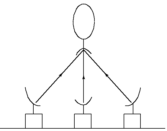
Suppose that
m stations wish to communicate with a common satellite over a common channel, as shown in
1↓. This is known as a
multiple-access channel.
How do the various senders cooperate with each other to send information to the receiver? What rates of communication are achievable simultaneously? What limitations does interference among the senders put on the total rate of communication? This is the best understood mutiuser channel, and the above questions have satisfying answers.
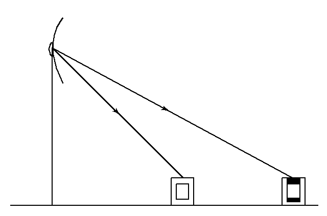
In contrast, we can reverse the network and consider one TV station sending information to
m TV receivers, as in
2↓.
How does the sender encode information meant for different receivers in common signal? For this channel, the answers are known only in special cases. There are other channels, such as the relay channel where there is one source and one destination, but one or more intermediate sender-receiver pairs that achts as relays to facilitate the communications between the source and the destination), the interference channel (two senders and two receivers with crosstalk), and the two-way channel (two sender-receiver pairs sending information to each other). For all these channels, we have only some of the answers to questions about achievable communication rates and the appropriate coding strategies.
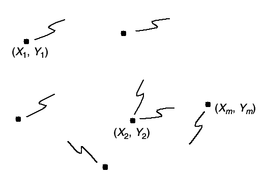
All these channels can be considered special cases of a general communication network that consists of
m nodes trying to communicate with each other, as shown in
3↓.
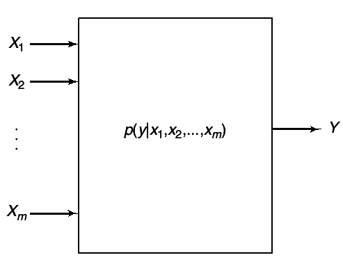
At each instant of time, the i -th node sends a symbol xi that depends on the messages that it wants to send and the past received symbols at the node. The simultaneous transmission of the symbols (x1, x2, ..., xm) resulsts in random received symbols (Y1, Y2, ...Ym) drawn according to the conditonal probability distribution p(y(1), y(2), ..., y(m)|x(1), x(2), ..., x(m)). Here p(⋅|⋅) expresses the effects of the noise and interference present in the network. If p(⋅|⋅) takes only the values 0 and 1 ,the network is deterministic.
Associated with some of the nodes in the network are stochastic data sources, which are to be communicated to some of the other nodes in the network. If the sources are independent, the messages sent by the nodes are also independent. However, for full generality, we must allow the sources to be dependent. How does one take advantage of the dependence to reduce the amount of information transmitted? Given the probability distribution of the sources and the channel transition function, can one transmit these sources over the channel and recover the sources at the destinations with the appropriate distortion?
We consider various special cases of network communication. We consider the problem of source coding when the channels are noiseless and without interference. In such cases, the problem reduces to finding the set of rates associated with each source such that the required sources can be decoded at the destination with a low probability of error (or appropriate distortion). The simplest case for distributed source coding is the Slepian-Wolf source coding problem, where we have two sources that must be encoded separately, but decoded together at common node. We consider extensions to this theory when only one of the two sources needs to be recovered at the destination.
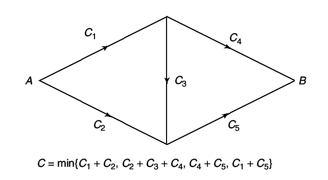
The theory of flow in networks has satisfying answers in such domains as circuit theory and the flow of water in pipes. For example, for the single-source single-sink network of pipes shown in
4↓, the maximum flow form
A to
B can be computed easily from the Ford-Fulerson theorem.
Assume that the edges have capacities Ci as shown. Clearly, the maximum flow across any cut set cannot be greater than the sum of the capacities of the cut edges. Thus minimizing the maximum flow across cut sets yields an upper bound on the capacity of the network. The Ford-Flulkerosn Theorem shows that this capacity can be achieved.
The theory of information flow in networks doesn’t have the sae simple answer as the theory of flow of water in pipes. Allthough we prove an upper bound on the rate of informaion flow across any cut set, these bounds are not achievable in general. However, it is gratifying that some problems, such as the relay channel and the cascade channel, admit a simple max-flow min-cut interpretation. Another subtle problem in the seach for general theory is the absence of a source-channel separation theorem, which we touch on briefly in Section 15.10. A complete theory combining distributed source coding and network channel coding is still distant goal.
In the next section we consider Gaussian examples of some of the basic channels of network information theory. The physically motivated Gaussian channel lends itself to concrete and easily interpreted answers. Later we prove some of the basic results about joint typicality that we use to prove the theorems of multiuser information theory. We then consider various problems in detail: the multiple-access channel, the coding of correlated sources (Slepian-Wolf data compression), the broadcast channel, the relay channel, the coding of a random variable with side information, and the rate distortion problem with side information. We end with an introduction to the general theory of informaion flow in networks. There are a number of open problems in the area, and there does not yet exist a comprehensive theory of information networks. Even if such a theory is found, it may be too complex for easy implementation. But the theory will be able to tell communication designers how close they are to optimality and perhaps suggest some means of improving the communication rates.
1.1 Gaussian Multiple-user channels
Gaussian multiple-user channels illustrate some of the important features of network information theory. The intuition gained in Chapter 9 on the Gaussian channel should make this section a useful introduction. Here the key ideas for establishing the capacity regions of the Gaussian multiple access, broadcast, relay, and two-way channels will be given without proof. The proofs of the coding theorems for the discrete memory-less counterparts to these theorems are given in letter sections of the chapter.
The basic discrete-time additive white Gaussian noise channel with input power P and noise variance N is modeled by:
where the Zi are i.i.d Gaussian random variables with mean 0 and variance N. The signal X = (X1, X2, ..., Xn) has power constraint
The Shannon capacity C is obtained by maximizing I(X;Y) over all random variables X such that EX2 ≤ P and is given by
In this chapter we restrict our attention to discrete-time memoryless channels; the results can be extended to continuous-time Gaussian channels.
1.1.1 Single-User Gaussian Cahnnel
We first review the single-user Gaussian channel studied in Chapter 9. Here Y = X + Z. Chose a rate R < (1)/(2)⋅log⎛⎝1 + (P)/(N)⎞⎠. Fix a good (2nR, n) codebook of power P. Choose an index w in the set 2nR. Send the w-th codeword X(w) from the code-book generated above. The receiver observes Y = X(w) + Z and then finds the index ŵ of the codeword closest to Y. If n is sufficiently large, the probability of error Pr(w ≠ ŵ) will be arbitrarily small. As can be seen form the definition of joint typicality, this minimum-distance decoding scheme is essentially equivalent to finding the codeword in code-book that is jointly typical with the received vector Y.
1.1.2 Gaussian Multiple-Access Channel with m Users
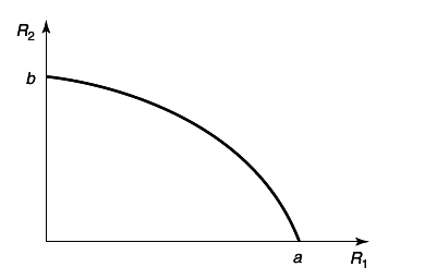
We consider m transmitters each with a power P. Let
Let
denote the capacity of a single-user Gaussian channel with signal to noise ratio (P)/(N) . The achievable rate region for the Gaussian channel takes on the simple form given in the following equations:
Note that when all the rates are the same, the last inequality dominates the others.
Here we need m codebooks, the i-th codebook having 2nRi codewords of power P. Here we need m codebooks, the i-th codebook having 2nRi codewords of power P . Transmission is simple. Each of the independent transmitters chooses an arbitrary codeword form its own codebook. The users send the vectors simultaneously. The receiver sees the codewors added together with the Gaussian noise Z.
Optimal decoding consists of looking for the m codewords, one from each codebook, such that the vector sum is closest to Y in euclidean distance. If (R1, R2, ...Rm) is in the capacity region given above, the probability of error goes to 0 as n tends to infinity.
It is exiting to see in this problem that the sum of the rates of the users C(mP ⁄ N) goes to infinity with m. Thus, in a cocktail party with m celebrants of power P in the presence of ambient noise N, the intended listener receives an unbounded amount of information as the number of people grows to infinity. A similar conclusion holds, of course, for ground communications to a satellite. Apparently, the increasing interference as the number of senders m → ∞ does not limit the total received information.
It is also interesting to note that the optimal transmission scheme here does not involve time-division multiplexing. In fact, each of the transmitters uses all of the bandwidth all of the time.
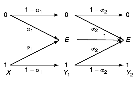
1.1.3 Gaussian Broadcast Channel
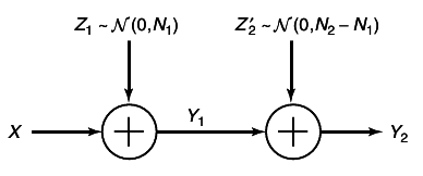
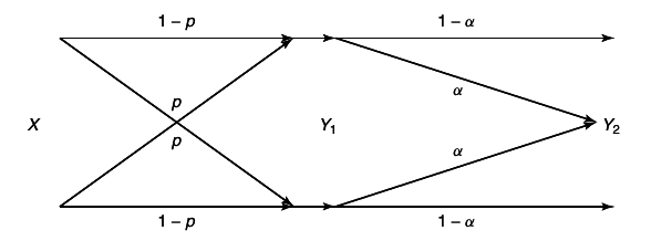
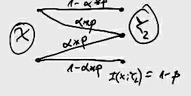
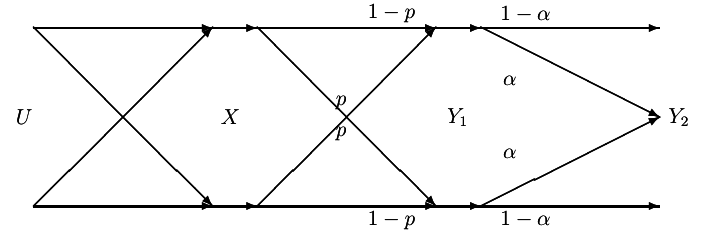
Here we assume that we have a sender of power P and two distant receivers, one with Gaussian noise power N1 and the other with Gaussian noise power N2. Without loss of generality, assume that N1 < N2. Thus, receiver Y1 is less noisy than receiver Y2. The model for the channel is Y1 = X + Z1 and Y2 = X + Z2, where Z1 and Z2 are arbitrarily correlated Gaussian random variables with variances N1 and N2, respectively. The sender wishes to send independent messages at rates R1 and R2 to receivers Y1 and Y2, respectively.
Fortunately, all scalar Gaussian broadcast channels belong to the class of degraded broadcast channels discussed in Section 15.6.2. Specializing that work, we find that the capacity region of the Gaussian broadcast channel is:
where α may be arbitrarily chosen (0 ≤ α ≤ 1) to trade off rate R1 for rate R2 as transmitter wishes.
To encode the messages, the transmitter generates two codebooks, one with power αP at rate R1, and another codebook with power αP
α = 1 − α
at rate R2, where R1 and R2 lie in the capacity region above. Then to send an index w1 ∈ {1, 2, ...2nR1} and w2 ∈ {1, 2, ..2nR2} to Y1 and Y2, respectively, the transmitter takes the codeword X(w1) from the first codebook and codeword X(w2) from the second codebook and computes the sum. He sends the sum over the channel.
The receivers must now decode the messages. First consider the bad receiver Y2. He merely looks through the second codebook to find the closest codeword to the received vector Y2. His effective signal-to-noise ratio is αP ⁄ (αP + N2), since Y1 's message acts as noise to Y2. (This can be proved).
The good receiver Y1 first decodes Y2 's codeword, which he can accomplish because of his lower noise N1. He subtracts this codeword X̂2 from Y1. He then looks for the codeword in the first codebook closest to Y1 − X̂2. The resulting probability of error can be made as low as desired.
A nice dividend of optimal encoding for degraded broadcast channels is that the better receiver Y1 always knows the message intended for receiver Y2 in addition to the message intended for himself.
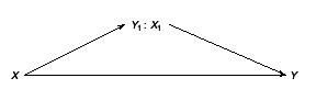
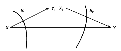
1.1.4 Gaussian Relay Channel
For the relay channel, we have a sender
X and an ultimate intended receiver
Y. Also present is the relay channel, intended solely to help the receiver. The Gaussian relay channel
5↓ is given by
where Z1 and Z2 are independent zero-mean Gaussian random variables with variance N1 and N2, respectively. The encoding allowed by the relay is the causal sequence
Sender X has power P and sender X1 has power P1. The capacity is
where α = 1 − α. Note that if
(P + P1 + 2√(αPP1))/(N1 + N2) = ((√(αP) + √(P1))2)/(N1 + N2) = (√((αP)/(N1 + N2)) + √((P1)/(N1 + N2)))2 =
= ||P1 ≥ (N2P)/(N1), || ≥ (√((αP)/(N1 + N2)) + √((N2P)/(N1(N1 + N2))))2 =
= (αP⋅N1)/(N1(N1 + N2)) + (N2P)/(N1(N1 + N2)) + 2√((αP)/(N1 + N2)⋅(N2P)/(N1(N1 + N2))) = ((αN1 + N2)P)/(N1(N1 + N2)) + 2(P√(αN1N2))/(N1(N1 + N2)) =
= ((αN1 + N2)P + 2P√(αN1N2))/(N1(N1 + N2)) = ((√(αN1) + √(N2))2P)/(N1 + N2) ≥ |α = 1| ≥ (N1 + 2√(N1N2) + N2)/(N1(N1 + N2))⋅P = ⎛⎝1 + 2(√(N1N2))/(N1 + N2)⎞⎠(P)/(N1) ≥ (P)/(N1)
It can be seen that C = C(P ⁄ N1),
Доказот е во Box-от погоре!!!
which is achieved by α = 1. The channel appears to be noise-free after the relay, and the capacity C(P ⁄ N1) from X to the relay can be achieved. Thus, the rate C(P ⁄ (N1 + N2)) without the relay is increased by the presence of the relay to C(P ⁄ N1). For large N2 and for P1 ⁄ N2 ≥ P ⁄ N1, we see that the increment in rate is form C(P ⁄ N1 + N2) ~ 0 to C(P ⁄ N1).
Let R1 < C⎛⎝(αP)/(N1)⎞⎠. Two codebooks are needed. The first codebook has 2nR1 words of power αP. The second has 2nR0 codewords of power αP. We shall use codewords form these codebooks successively to create the opportunity for cooperation by the relay. We start by sending a codeword from the first codebook. The relay now knows the index of this codeword since R1 < C(αP ⁄ N1), but the intended receiver has a list of possible codewords of size 2n(R1 − C(αP ⁄ (N1 + N2)))
Не контам од каде излегуа ова!? Ска да каже дека реалниот капацитет е разлика меѓу капацитетот меѓу предавателот и релето и капацитетот кога не би постоело релето.
. This list calculation involves a result on list codes.
M = 2nR; nR = logM; R = (1)/(n)logM; R ≤ C; (1)/(n)logM ≤ C; M ≤ 2nC
In the next block, the transmitter and the relay wish to cooperate to resolve the receiver’s uncertainty about the codeword sent previously that is on the receiver’s list. Unfortunately, they cannot be sure what this list is because they do not know the received signal Y. Thus, they randomly partition the first codebook into 2nR0 cells with and equal number of codewords in each cell. The relay, the receiver, and the transmitter agree on this partition. The relay and the transmitter find the cell of the partiotion in which the codeword from the first codebook lies and cooperatively send the codeword form second codebook with that index. That is, X and X1 send the same designated codeword. The relay, of course, must scale this codeword so that it meet his power constraint P1. They now transmit their codewords simultaneously. An important point to note here is that the cooperative information sent by the relay and the transmitter is sent coherently. So the power of the sum as seen by the receiver Y is (√(α)P + √(P1))2.
However, this does not exhaust what the transmitter does in the second block. He also chooses a fresh codeword from the first codebook, adds it „on paper” to the cooperative codeword form the second codebook, and sends the sum over the channel. The reception by the ultimate receiver Y in the second block involves first finding the cooperative index from the second codebook by looking for the closest codeword in the second codebook. He subtracts the codeword form the received sequence and then calculates a list of indices of size 2nR0 corresponding to all codewords of the first codebook that might have been sent in the second block.
Now it is time for the intended receiver to complete computi9ng the codeword form the first codebook sent in the first blcok. He takes his list of possible codewords that might have been sent in the first block and intersects it with the cell of the partition that he has learned form the cooperative relay transmission in the second block. The rates and powers have been chosen so that there is only one codeword in the intersection. This is Y’s guess about the information sent in the first block.
We are now in steady state. In each new block, the transmitter and the relay cooperate to resolve the list uncertainty form the previous block. In addition, the transmitter superimposes some fresh information from his first codebook to thistransmission form the second codebook and transmits the sum. The receiver is always one block behind, but for sufficiently many blocks, this does not affect his overall rate of reception.
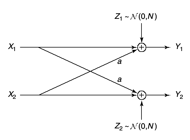
1.1.5 Gaussian Interference Channel
The interference channel has two senders and two receivers. Sender 1 wishes to send information to receiver 1. He does not care what receiver 2 receives or understands; similarly with sender 2 and receiver 2. Each channel interferences with the other. This channel is illustrated in
6↓.
It is not quite a broadcast channel since there is only one intended receiver for each sender, nor is it a multiple access channel because each receiver is only interested in what is being sent by the corresponding transmitter.
For symmetric interference, we have
where Z1, Z2 are independent N(0, N) random variables. This channel has not been solved in general even in Gaussian case. But remarkably, in the case of high interference, it can be shown that the capacity region of this channel is the same as if there were no interference whatsoever.
To achieve this, generate two codebooks, each with power P and rate C(P|N). Each sender independently chooses a word from his book and sends it. Now, if the interference a satisfies C(a2P ⁄ (P + N)) > C(P ⁄ N), the first transmitter understands perfectly the index of second transmitter. He finds it by the usual technique of looking for the closest codeword to his received signal. Once he finds this signal, he subtracts it form his waveform received. Now there is a clean channel between him and his sender. He then searches the sender’s codebook to find the closest codeword and declares that codeword to be the one sent.
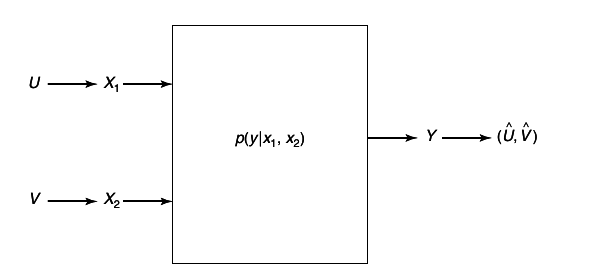
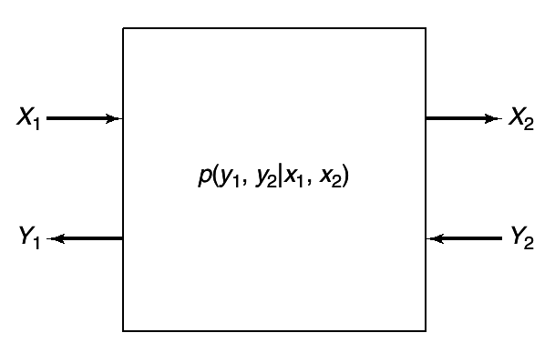
1.1.6 Gaussian Two-way channel
The two-way channel is very similar to the interference channel, with the additional provision that sender 1 is attached to receiver 2 and sender 2 is attached to receiver 1, as shown in
7↓. Hence, sender 1 can use information from previous received symbols of receiver 2 to decide what to send next. This channel introduces another fundamental aspect of network information theory: namely feedback. Feedback enables the senders to use the partial information that each has about the other’s message to cooperate with each other.
The capacity region of the two-way channel was considered by Shannon
[3], who derived upper and lower bounds on the region (Seе Problem 15.15). For Gaussian channels, these two bounds coincide and the capacity region is known; in fact, the Gausisian two-way channel decomposes into two independent channels.
Let P1 and P2 be the powers of transmitters 1 and 2, respectively, and let N1 and N2 be the noise variances of the two channels. Then the rates R1 < C(P1|N1) and R2 < C(P2|N2) can be achieved by the techniques described for the interference channel. In this case, we generate two codebooks of rates R1 and R2. Sender 1 sends a code-word from the first codebook. Receiver 2 receives the sum of the codewords sent by the two senders plus some noise. He simply subtracts out the code out the codeword of sender 2 and he has a clean channel form sender 1 (with only the noise of variance N1). Hence the two-way Gaussian channel decomposes into two independent Gaussian channels. But this is not the case for the general two-way channel; in general, there is a trade-off between the two senders so that both of them cannot send at the optimal rate at the same time.
1.2 Jointly Typical sequences
We have previewer the capacity results for networks by considering multiuser Gaussian channels. We began a more detailed analysis in this section, where we extend the joint AEP provided in Chapter 7 to a form that we will use to prove the theorems of network information theory. The joint AEP will enable us to calculate the probability of error for jointly typical decoding for the various coding schemes considered in this chapter.
Let (X1, X2, ..., Xk) denote a finite collection of discrete random variables with some fixed joint distribution, p(x(1), x(2), ..., x(k)), (x(1), x(2), ..., x(k)) ∈ X1 xX2 x...xXk. Let S denote an ordered subset of these random variables and consider n independent copies of S. Thus,
For example, if S = (Xj, Xl), then
Pr{S = s} = Pr{(Xj, Xl) = (xj, xl)} = n∏i = 1p(xij, xil)
X1 ∈ (0, 1), p(X1) = ⎧⎩(1)/(2), (1)/(2)⎫⎭; X2 ∈ (0, 1), p(X2) = ⎧⎩(1)/(2), (1)/(2)⎫⎭;
n = 3
S = (X1, X2)
Pr{S = s} = Pr{(X1, X2) = ( x1, x2) = (x11x21x31, x12x22x32)} = ∏3i = 1p(xi1, xi2) =
= p(x11, x12)p(x21x22)p(x31x32)
To be explicit, e will sometimes use X(S) for S. By the law of large numbers, for any subset S of random variables,
where the convergence takes place with probability 1 for all 2k subsets S ⊆ {X(1), X(2), ..., X(k)}.
Definition (
ϵ-typical
n-sequences)
The set A(n)ϵ of ϵ-typical n-sequences (x1, x2, ..., xk) is defined by:
A(n)ϵ(X(1), X(2), ..., X(k)) = A(n)ϵ = ⎧⎩(x1, x2, ..., xk):|| − (1)/(n)logp(s) − H(S)|| < ϵ, ∀S ⊆ {X(1), X(2), ..., X(k)}⎫⎭
Аналогијата е дека X(1) одговара на Xn, a X(2) на Yn и така натака...
Let A(n)ϵ(S) denote the restriction of A(n)ϵ to the coordinates of S. Thus, if S = (X1, X2), we have
A(n)ϵ(X1, X2) = ⎧⎩(x1, x2):|| − (1)/(n)logp(x1, x2) − H(X1, X2)|| < ϵ, || − (1)/(n)logp(x1) − H(X1)|| < ϵ, || − (1)/(n)logp(x2) − H(X2)|| < ϵ⎫⎭
We will use the notation αn≐2n(b±ϵ) to mean that
for n sufficiently large.
Внимавај нема − пред (1)/(n) како во стандардната дефиниција на AEP
For any
ϵ > 0, for sufficiently large
n,
2. s ∈ A(n)ϵ(S) ⇒ p(s)≐2 − n(H(S)±ϵ).
3. \mathchoice|A(n)ϵ(S)|≐2n(H(S)±2ϵ).|A(n)ϵ(S)|≐2n(H(S)±2ϵ).|A(n)ϵ(S)|≐2n(H(S)±2ϵ).|A(n)ϵ(S)|≐2n(H(S)±2ϵ).
1. This follows form the law of large numbers for the random variable in the definition A(n)ϵ(S).
2. This follows directly from the definition of A(n)ϵ(S).
3. This follows form
→ |A(n)ϵ| ≤ 2 + n(H(S) + ϵ)
→ |A(n)ϵ| ≥ (1 − ϵ)2 + n(H(S) − ϵ)
(1 − ϵ)⋅2n(H(S) − ϵ) ≤ |A(n)ϵ| ≤ 2n(H(S) + ϵ)
Combining
25↑ and
24↑ we have
\mathchoice|A(n)ϵ|≐2n(H(S1)±2ϵ)|A(n)ϵ|≐2n(H(S1)±2ϵ)|A(n)ϵ|≐2n(H(S1)±2ϵ)|A(n)ϵ|≐2n(H(S1)±2ϵ) for sufficiently large
n.
(1 − ϵ)⋅2 + n(H(S) − ϵ) ≤ |A(n)ϵ| ≤ 2n(H(S) + ϵ) 2 + n(H(S) − ϵ) − ϵ⋅2 + n(H(S) − ϵ) ≤ |A(n)ϵ| ≤ 2n(H(S) + ϵ)
2 + n(H(S) − ϵ) ≤ |A(n)ϵ| + ϵ⋅2 + n(H(S) − ϵ) ≤ 2n(H(S) + ϵ)
\mathchoice||(1)/(n)logan − b|| < ϵ αn≐2n(b±ϵ);||(1)/(n)logan − b|| < ϵ αn≐2n(b±ϵ);||(1)/(n)logan − b|| < ϵ αn≐2n(b±ϵ);||(1)/(n)logan − b|| < ϵ αn≐2n(b±ϵ); − ϵ < − (1)/(n)logan − b < ϵ b − ϵ < − (1)/(n)logan < b + ϵ
n⋅(b − ϵ) < − logan < n(b + ϵ)
− n(b − ϵ) > logan > − n(b + ϵ) 2 − n(b + ϵ) ≤ an ≤ 2 + n(b − ϵ)
(1 − ϵ)⋅2n(H(S) − ϵ) ≤ |A(n)ϵ| ≤ 2n(H(S) + ϵ)
log(1 − ϵ) + n(H(S) − ϵ) ≤ log|A(n)ϵ| ≤ n(H(S) + ϵ)
(1)/(n)log(1 − ϵ) + (H(S) − ϵ) ≤ (1)/(n)log|A(n)ϵ| ≤ (H(S) + ϵ)
——————————————————————————–——————————————————————————–——————————
− (1)/(n)log(1 − ϵ) − (H(S) − ϵ) ≥ − (1)/(n)log|A(n)ϵ| ≥ − H(S) − ϵ;
− (1)/(n)log(1 − ϵ) − ϵ ≥ − (1)/(n)log|A(n)ϵ| ≥ − H(S) − ϵ
——————————————————————————–——————————————————————————–——————————
\cancelto − ϵ(1)/(n)log(1 − ϵ) − ϵ ≤ (1)/(n)log|A(n)ϵ| − H(S) ≤ ϵ
-2ϵ ≤ (1)/(n)log|A(n)ϵ| − H(S) ≤ ϵ \strikeout off\uuline off\uwave offAко важи за ϵ ќе важи и за2ϵ
− 2ϵ ≤ (1)/(n)log|A(n)ϵ| − H(S) ≤ 2ϵ → ||(1)/(n)log|A(n)ϵ| − H(S)|| ≤ 2ϵ → |A(n)ϵ|≐2n(H(S)±2ϵ)
Dокажано!!!
4. Let S1, S2 ⊆ {X(1), X(2), ..., X(k)}If (s1, s2) ∈ A(n)ϵ(S1, S2)then p(s1|s2) = 2 − n(H(S1|S2)±2ϵ)
For (s1, s2) ∈ A(n)ϵ(S1, S2) we have p(s1)≐2 − n(H(S1)±ϵ) and p(s1, s2)≐2 − n(H(S1S2)±ϵ) hence
p(s2| s1) = (p(s1, s2))/(p(s1)) = (2 − n(H(S1S2)±ϵ))/(2 − n(H(S1)±ϵ))≐2 − n(H(S1S2) − H(S1)±ϵ)≐2 − n(H(S2|S1)±2ϵ)
The next theorem bounds the number of conditionally typical sequences for a given typical sequence.
Let S1S2 be two subsets of X(1), X(2), ..., X(k). For any ϵ > 0, define A(n)ϵ to be the set of s1 sequences that are jointly ϵ-typical with a particular s2 sequence. If s2 ∈ A(n)ϵ(S2), then for sufficiently large n, we have
\mathchoice|A(n)ϵ(S1| s2)| ≤ 2n(H(S1|S2) + 2ϵ)|A(n)ϵ(S1| s2)| ≤ 2n(H(S1|S2) + 2ϵ)|A(n)ϵ(S1| s2)| ≤ 2n(H(S1|S2) + 2ϵ)|A(n)ϵ(S1| s2)| ≤ 2n(H(S1|S2) + 2ϵ)
and
\mathchoice(1 − ϵ)2n(H(S1|S2) − 2ϵ) ≤ ⎲⎳s2p(s2)|A(n)ϵ(S1| s2)|(1 − ϵ)2n(H(S1|S2) − 2ϵ) ≤ ⎲⎳s2p(s2)|A(n)ϵ(S1| s2)|(1 − ϵ)2n(H(S1|S2) − 2ϵ) ≤ ⎲⎳s2p(s2)|A(n)ϵ(S1| s2)|(1 − ϵ)2n(H(S1|S2) − 2ϵ) ≤ ⎲⎳s2p(s2)|A(n)ϵ(S1| s2)|
As in part 3 of Theorem 15.2.1, we have
If
n is sufficiently large we, can argue form
22↑ that
1 − ϵ ≤ \mathchoice ⎲⎳s2p(s2) ⎲⎳s1 ∈ Anϵ(S1| s2)p(s2| s1) ⎲⎳s2p(s2) ⎲⎳s1 ∈ Anϵ(S1| s2)p(s2| s1) ⎲⎳s2p(s2) ⎲⎳s1 ∈ Anϵ(S1| s2)p(s2| s1) ⎲⎳s2p(s2) ⎲⎳s1 ∈ Anϵ(S1| s2)p(s2| s1) ≤ ⎲⎳s2p(s2) ⎲⎳s1 ∈ Anϵ(S1| s2)2 − n(H(S1|S2) − 2ϵ) = ⎲⎳s2p(s2)⋅A(n)ϵ(S1| s2)⋅2 − n(H(S1|S2) − 2ϵ)
= 2 − n(H(S1|S2) − 2ϵ)⋅ ⎲⎳s2p(s2)⋅A(n)ϵ(S1| s2)
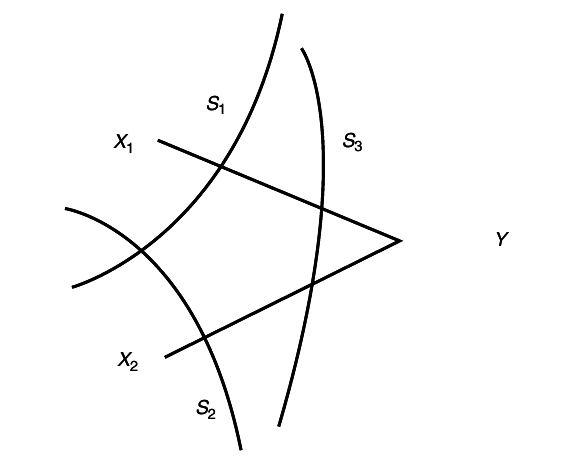
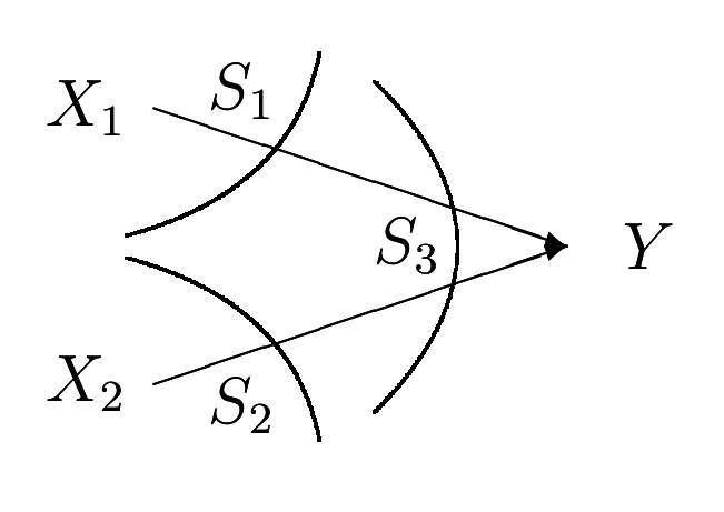
To calculate the probability of decoding error, we need to know the probability that conditionally independent sequences are jointly typical. Let S1S2, and S3 be three subsets of {X(1), X(2), ...X(k)}. If S’1 and S’2 are conditionally independent given S3’ but otherwise share the same pairwise marginals of (S1, S2, S3) we have the following probability of joint typicality.
Let A(n)ϵ denote the typical set for the probability mass function p(s1s2s3) and let
Then
P{S1’, S2’, S3’ ∈ A(n)ϵ}≐2 − n(I(S1;S2|S3)±6ϵ)
We use the
≐ notation form
21↑ to avoid calculating the upper and lower bounds separately. We have
P{(S1’, S2’, S3’) ∈ A(n)ϵ} = ⎲⎳(s1, s2, s3) ∈ A(n)ϵp(s3)p(s1|s3)p(s2|s3)≐|A(n)ϵ(S1S2S3)|2 − n(H(S3)±2ϵ)2 − n(H(S1|S3)±2ϵ)2 − n(H(S2|S3)±2ϵ)
≐2n(H(S1S2S3)±ϵ) − n(H(S3)±ϵ) − n(H(S1|S3)±2ϵ) − n(H(S2|S3)±2ϵ)≐2 − n(I(S1;S2|S3)±6ϵ)
Во книгата е 2 − n(I(S1;S2|S3)±6ϵ) но мене ми излегува со 2ϵ затоа што ги земам во предвид промените на знаците на ± . Ако не се земат во предвид тие промени тогаш се добива 6ϵ.
n(H(S1S2S3)±ϵ) − n(H(S3)±ϵ) − n(H(S1|S3)±2ϵ) − n(H(S2|S3)±2ϵ) =
n[H(S1S2S3)±ϵ − H(S3)∓ϵ − H(S1|S3)∓2ϵ − H(S2|S3)∓2ϵ]
n[H(S1S2S3) − H(S3) − H(S1|S3) − H(S2|S3)] = (*)
I(S1;S2|S3) = H(S1|S3) − H(S1|S2S3)
H(S1S2S3) = H(S3) + H(S2|S3) + H(S1|S2S3)
(*) = n[\cancelH(S3) + \cancelH(S2|S3) + H(S1|S2S3) − \cancelH(S3) − H(S1|S3) − \cancelH(S2|S3)] = − n⋅I(S1;S2|S3)
Ако се земат во предвид проментие на знаците во ± тогаш:
n[H(S1S2S3)±ϵ − H(S3)∓ϵ − H(S1|S3)∓2ϵ − H(S2|S3)∓2ϵ] = − n⋅(I(S1;S2|S3)±4ϵ)
Ако не се земат во предвид промените на знаците во ± тогаш:
n[H(S1S2S3)±ϵ − H(S3)±ϵ − H(S1|S3)±2ϵ − H(S2|S3)±2ϵ] = − n⋅(I(S1;S2|S3)±6ϵ)
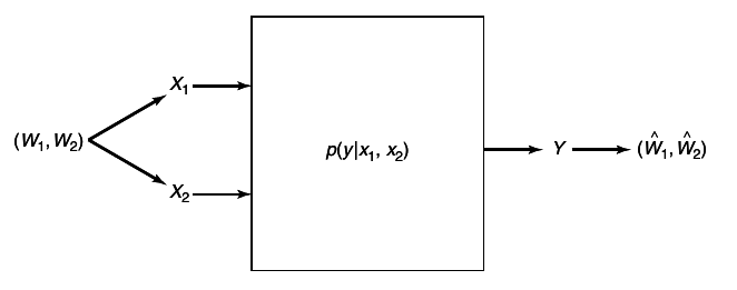
1.3 Multiple-access channel
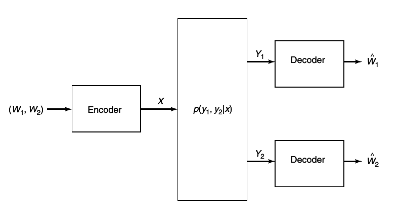
The fist channel that we examine in detail is the multiple-access channel, in which two (or more) senders send information to a common receiver. The channel is illustrated in
10↓.\begin_inset Separator latexpar\end_inset
A common example of this channel is a satellite receiver with many independent ground stations, or a set of cell phones communicating with a base station. We see that the senders must contend not only with the receiver noise but with interference from each other as well.
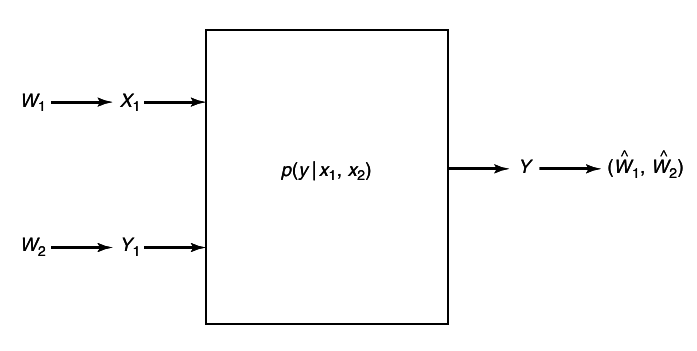
A discrete memory-less multiple-access channel consists of three alphabets , X1, X2 and Y, and a probability transition matrix p(y|x1, x2).
Definition (average probability of error)
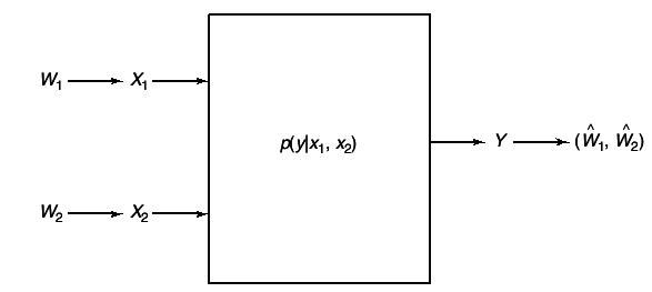
A ((2nR12nR2), n) code for the multiple-access channel consists of two sets of integers W1 = {1, 2, ..., 2nR1} and W2 = {1, 2, ...2nR2} called message sets, two encoding functions,
and
and a decoding function,
There are two senders and one receiver for this channel. Sender 1 chooses an index W1 uniformly form the set {1, 2, ..., 2nR1} and sends the corresponding codeword over the channel. Sender 2 does likewise. Assuming that the distribution of messages over the product set W1 xW2 is uniform (i.e. the messages are independent and equally likely), we define the average probability of error for the ((2nR1, 2nR2), n) code as follows:
P(n)e = (1)/(2n(R1 + R2))⋅ ⎲⎳(w1, w2) ∈ W1 xW2Pr{g(Yn) ≠ (w1w2)|(w1w2) sent}
Definition (achievable rate pair)
A rate pair (R1, R2) is said to be achievable for the multiple access channel if there exists a sequence of ((2nR1, 2nR2), n) codes with P(n)ϵ → 0.
The capacity region of the multiple-access channel is the closure of the set of achievable (R1R2) rate pairs.
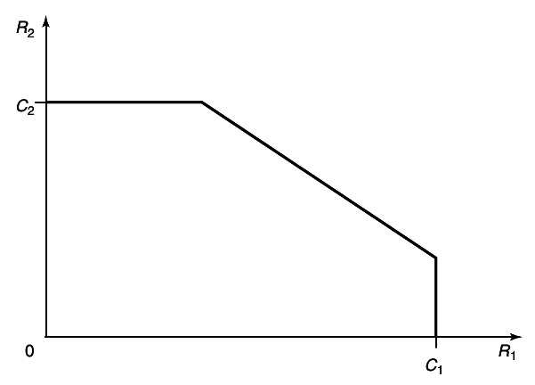
An example of the capacity region for a multiple-access channel is illustrated in figure 4
11↓. We first state the capacity region in the form of a theorem.
Theorem 15.3.1 (Multiple-access channel capacity)
The capacity of a multiple-access channel (X1 xX2, p(y|x1, x2), Y) is the closure of the convex hull of all (R1R2) satisfying
for some product distribution p2(x1)p2(x2) on X1 xX2.
Дефиниција од B. Grunbaum, Convex Polytopes за конвексна лушпа (convex hull) е: The convex hull conv(A) of subset A of Rd is the intersection of all the convex sets in Rd which contain A .
Before we prove that this is the capacity region of the multiple-access channel, let us consider a few examples of multiple-access channels:
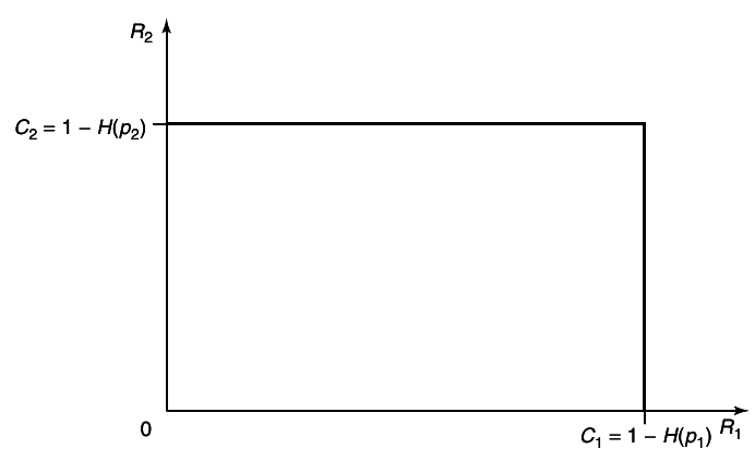
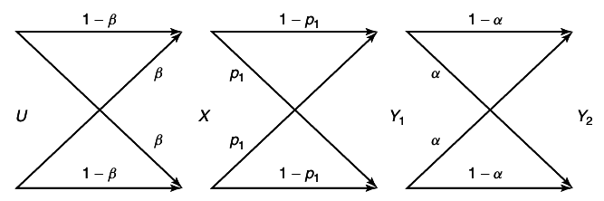
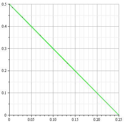
Example 15.3.1 (Independent binary symmetric channel)
Assume that we have two independent binary symmetric channels one from sender 1 and other from sender 2 as shown in
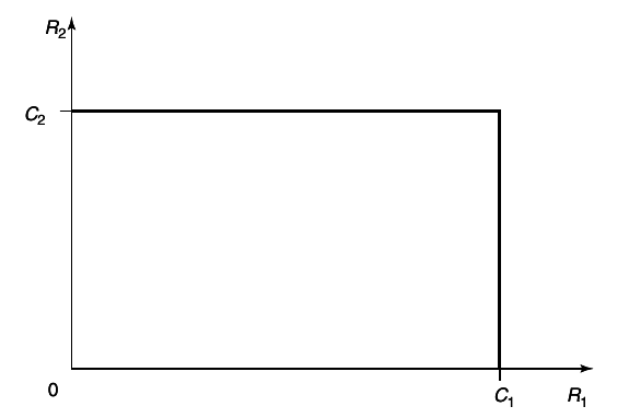
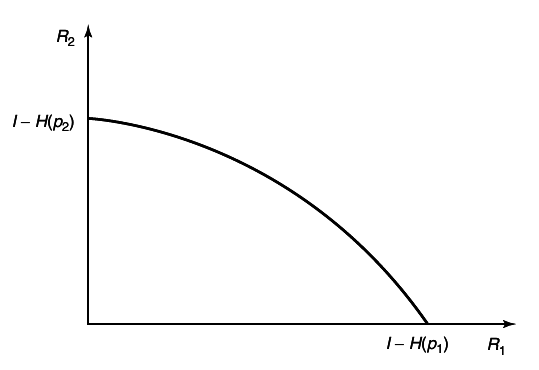
12↓. In this case, it is obvious from the results of Chapter 7 that we can sent at rate
1 − H(p1) over the first channel and at rate
1 − H(p2) over the second channel. Since the channels are independent, there is no interference between the senders. The capacity region in this case is shown in
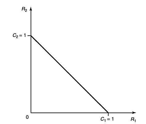
Example 15.3.2 (Binary multiplier channel)
Consider a multiple-access channel with binary inputs and outputs
Such channel is called
binary multiplier channel. It is easy to see that by setting
X2 = 1, we can send at a rate of
1 bit per transmission form sender
1 to the receiver. Similarly, setting
X1 = 1, we can achieve
R2 = 1. Clearly, since the output is binary, the combined rates
R1 + R2 cannot be more that 1 bit.
By time-sharing, we can achieve any combination of rates such that R1 + R2 = 1. Hence the capacity region is shown in
14↓
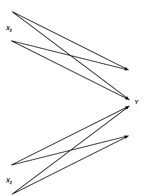
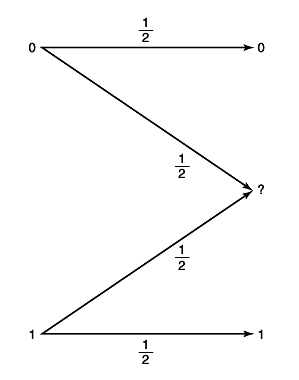
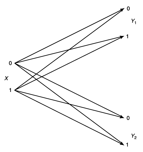
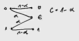
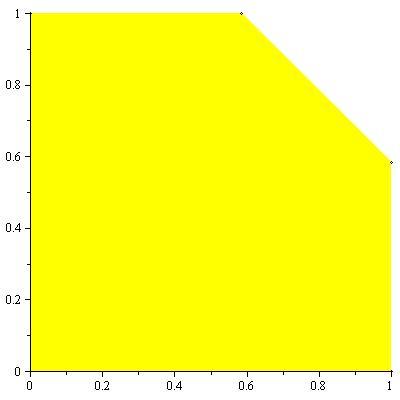
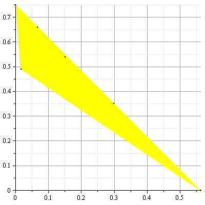
Example 15.3.3 (Binary erasure multiple-access channel)
This multiple-access channel has binary inputs, X1 = X2 = {0, 1} and ternary output Y = X1 + X2. There is no ambiguity in (X1X2) if Y = 0 or Y = 2 is received; but Y = 1 can result form either (0, 1) or (1, 0).
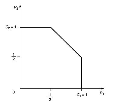
We now examine the achievable rates on the axes. Setting X2 = 0, we can send at rate of 1 bit per transmission from sender 1. Similarly, setting X1 = 0, we can send at a rate R2 = 1. This gives us two extreme point of the capacity region. Can we do better? Let us assume that R1 = 1, so that the codewords of X1 must include all possible binary sequences; X1 would look like a Bernoulli⎛⎝(1)/(2)⎞⎠ process. That acts as a noise for the transmission from X2.
Ова јас го замислувам како X1 да е поблиску до Y, a X2 подалеку. Со тоа во Y X1 без проблем се декодира, но воедно тој претставува шум за подалечниот X2.
For
X2, the channel looks like the channel in
15↑. This is the binary erasure channel of Chapter 7. Recall in the results, the capacity of this channel is
(1)/(2) bits per transmission.
Hence when sending at the maximum rate 1 for sender 1, we can send an additional (1)/(2) bit form sender 2. Latter , after deriving the capacity region, we can verify that these rates are the best that can be achieved. The capacity region for a binary erasure channel is illustrated in
16↓.
1.3.1 Achievability of the Capacity Region for the Multiple-Access Channel
We now prove the achievability of he rate region in Theorem 15.3.1; the proof of the converse will be left until the next section. The proof of achievability is very similar to the proof for the single-user channel. We therefore only emphasize the points at which the proof differs form the single-user case. We begin by proving the achievability of rate pairs that satisfy
33↑ for some fixed product distribution
p(x1)p(x2). In Section 15.3.3 we extend this to prove that all points in the convex hull of
33↑ are achievable.
Proof: (Achievability in Theorem 15.3.1)
Fix \mathchoicep(x1, x2) = p1(x1)p2(x2)p(x1, x2) = p1(x1)p2(x2)p(x1, x2) = p1(x1)p2(x2)p(x1, x2) = p1(x1)p2(x2)
Generate 2nR1 independent codewords X1(i), i ∈ {1, 2, ..., 2nR1} , of length n, generating each element i.i.d. ~∏ni = 1p1(x1i). Similarly, generate 2nR2 independent codewords X2(j), j ∈ {1, 2, ..., 2nR2}, generating each element i.i.d ~ ∏ni = 1p2(x2i). These codewords form the code-book which is revealed to sender and the receiver.
To send index i, sender 1 sends the codeword X1(i). Similarly, to send j sender 2 sends X2(j).
Let A(n)ϵ denote the set of typical (x1 x2, y) sequences. The receiver Yn chooses the pair (i, j) such that
if such a pair (i, j) exists and is unique; otherwise, an error is declared.
Analysis of the probability of error:
By the symmetry of the random code construction, the conditional probability of error does not depend on which pair of indices is sent. Thus, the conditional probability of error is the same as the unconditional probability of error.
Потсети се како е дефинирана условната веројатност на грешка во Chapter 7 и како е дефинирана веројантоста на грешка. Ако сите условни веројатности се исти тогаш вкупнтата веројантост на грешка е еднакава на условната веројатност на грешка.
So without loss of generality, we can assume that (i, j) = (1, 1) was sent.
We have an error if either the correct codewords are not typical with the received sequence or there is a pair of incorrect codewords that are typical with the received sequence. Define the events
Then by the union of events bound,
where P is the conditional probability given that (1, 1) was sent. From the AEP, P(Ec11) → 0. By Theorems 15.2.1 and 15.2.3, for i ≠ 1 we have
\mathchoiceP(Ei1)P(Ei1)P(Ei1)P(Ei1) = Pr((X1(i), X2(1), Y) ∈ A(n)ϵ) = ⎲⎳(x1, x2, y) ∈ A(n)ϵp(x1)p(x2, y) ≤ |A(n)ϵ|2 − n(H(X1) − ϵ)2 − n(H(X2Y) − ϵ)
≤ 2n(H(X1X2Y) + 2ϵ)2 − n(H(X1) − ϵ)2 − n(H(X2Y) − ϵ) = 2 − n(H(X1) − ϵ + H(X2Y) − ϵ − H(X1X2Y) − 2ϵ) =
= 2 − n(H(X1) − ϵ + H(X2Y) − ϵ − H(X1X2Y) − 2ϵ) =
= 2 − n(H(X1) + H(X2Y) − H(X1X2Y) − 4ϵ) = |check box bellow| = 2 − n(I(X1;X2Y) − 4ϵ)\overset(a) = \mathchoice2 − n(I(X1;Y|X2 − 4ϵ)2 − n(I(X1;Y|X2 − 4ϵ)2 − n(I(X1;Y|X2 − 4ϵ)2 − n(I(X1;Y|X2 − 4ϵ)
Од Теорема 15.2.3 следи
P(S1’ = s1, S2’ = s2, S3’ = s3) = ∏ni = 1p(s1i|s3i)p(s2i|s3i)p(s3i)
∑(x1, x2, y) ∈ A(n)ϵp(x1|y)p(x2|y)p(y) = ∑(x1, x2, y) ∈ A(n)ϵp(x1)p(x2, y)
∑(x1, x2, y) ∈ A(n)ϵp(x1, x2, y) = ∑(x1, x2, y) ∈ A(n)ϵp(x1, x2)p(y|x1x2) = ∑(x1, x2, y) ∈ A(n)ϵp(x1)p(x2)p(y|x1x2) = ∑(x1, x2, y) ∈ A(n)ϵp(x1)p(x2y|x1)
Всушност ако се има во предвид Theorem 15.2.3 и се замисли дека X2 = S3
\mathchoice∑(x1, x2, y) ∈ A(n)ϵp(x2)⋅p(y, x1| x2) = ∑(x1, x2, y) ∈ A(n)ϵp(x2)⋅p(x1| x2)p(y|x2) = ∑(x1, x2, y) ∈ A(n)ϵp(x1)⋅p(x2)p(y|x2) = ∑(x1, x2, y) ∈ A(n)ϵp(x1)p(x2, y)∑(x1, x2, y) ∈ A(n)ϵp(x2)⋅p(y, x1| x2) = ∑(x1, x2, y) ∈ A(n)ϵp(x2)⋅p(x1| x2)p(y|x2) = ∑(x1, x2, y) ∈ A(n)ϵp(x1)⋅p(x2)p(y|x2) = ∑(x1, x2, y) ∈ A(n)ϵp(x1)p(x2, y)∑(x1, x2, y) ∈ A(n)ϵp(x2)⋅p(y, x1| x2) = ∑(x1, x2, y) ∈ A(n)ϵp(x2)⋅p(x1| x2)p(y|x2) = ∑(x1, x2, y) ∈ A(n)ϵp(x1)⋅p(x2)p(y|x2) = ∑(x1, x2, y) ∈ A(n)ϵp(x1)p(x2, y)∑(x1, x2, y) ∈ A(n)ϵp(x2)⋅p(y, x1| x2) = ∑(x1, x2, y) ∈ A(n)ϵp(x2)⋅p(x1| x2)p(y|x2) = ∑(x1, x2, y) ∈ A(n)ϵp(x1)⋅p(x2)p(y|x2) = ∑(x1, x2, y) ∈ A(n)ϵp(x1)p(x2, y)
докажано!!!
Ова се докажува и без Теорема 15.2.3
p(y, x1, x2) = p(x2)⋅p(y, x1| x2) = p(x2)⋅p(y|x2)p(x1| x2y) = p(x2)⋅p(y|x2)p(x1)
ако се претпостави дека x1 не зависи од y (Тоа важи ако имаш марков ланец X1 → X2 → Y).
|A(n)ϵ(S)|≐2n(H(S)±2ϵ)
\mathchoiceI(X1;X2Y) = H(X2Y) − H(X2Y|X1) = H(X2Y) − H(X2Y|X1) − H(X1) + H(X1) = H(X1) + H(X2Y) − H(X1X2Y)I(X1;X2Y) = H(X2Y) − H(X2Y|X1) = H(X2Y) − H(X2Y|X1) − H(X1) + H(X1) = H(X1) + H(X2Y) − H(X1X2Y)I(X1;X2Y) = H(X2Y) − H(X2Y|X1) = H(X2Y) − H(X2Y|X1) − H(X1) + H(X1) = H(X1) + H(X2Y) − H(X1X2Y)I(X1;X2Y) = H(X2Y) − H(X2Y|X1) = H(X2Y) − H(X2Y|X1) − H(X1) + H(X1) = H(X1) + H(X2Y) − H(X1X2Y)
Where equivalence in (a) follows form the independence of X1 and X2, and consequently
I(X1;X2Y) = \cancelto0I(X1;X2) + I(X1;Y|X2) = I(X1;Y|X2)
Similarly, for j ≠ 1,
Во овој случај соласно теорема 15.2.3 ќе земеш X1 = S3
Од Теорема 15.2.3 следи
P(S1’ = s1, S2’ = s2, S3’ = s3) = ∏ni = 1p(s1i|s3i)p(s2i|s3i)p(s3i)
Всушност ако се има во предвид Theorem 15.2.3 и се замисли дека X2 = S3
\mathchoice∑(x1, x2, y) ∈ A(n)ϵp(x1)p(x2y|x1) = ∑(x1, x2, y) ∈ A(n)ϵp(x1)p(x2|x1)p(y|x1) = ∑(x1, x2, y) ∈ A(n)ϵp(x1)p(x2)p(y|x1) = ∑(x1, x2, y) ∈ A(n)ϵp(x2)p(x1, y)∑(x1, x2, y) ∈ A(n)ϵp(x1)p(x2y|x1) = ∑(x1, x2, y) ∈ A(n)ϵp(x1)p(x2|x1)p(y|x1) = ∑(x1, x2, y) ∈ A(n)ϵp(x1)p(x2)p(y|x1) = ∑(x1, x2, y) ∈ A(n)ϵp(x2)p(x1, y)∑(x1, x2, y) ∈ A(n)ϵp(x1)p(x2y|x1) = ∑(x1, x2, y) ∈ A(n)ϵp(x1)p(x2|x1)p(y|x1) = ∑(x1, x2, y) ∈ A(n)ϵp(x1)p(x2)p(y|x1) = ∑(x1, x2, y) ∈ A(n)ϵp(x2)p(x1, y)∑(x1, x2, y) ∈ A(n)ϵp(x1)p(x2y|x1) = ∑(x1, x2, y) ∈ A(n)ϵp(x1)p(x2|x1)p(y|x1) = ∑(x1, x2, y) ∈ A(n)ϵp(x1)p(x2)p(y|x1) = ∑(x1, x2, y) ∈ A(n)ϵp(x2)p(x1, y)
|A(n)ϵ(S)|≐2n(H(S)±2ϵ)
(a) I(X2;X1Y) = H(X1Y) − H(X1Y|X2) = H(X1Y) − H(X1Y|X2) − H(X2) + H(X2) = H(X2) + H(X1Y) − H(X1X2Y)
\mathchoiceP(Ei1)P(Ei1)P(Ei1)P(Ei1) = P((X1(i), X2(1), Y) ∈ A(n)ϵ) = ∑(x1, x2, y) ∈ A(n)ϵp(x2)p(x1, y) ≤ |A(n)ϵ|2 − n(H(X2) − ϵ)2 − n(H(X1Y) − ϵ)
≤ 2n(H(X1X2Y) + 2ϵ)2 − n(H(X2) − ϵ)2 − n(H(X1Y) − ϵ) = 2 − n(H(X2) − ϵ + H(X1Y) − ϵ − H(X1X2Y) − 2ϵ)
= 2 − n(H(X2) + H(X1Y) − H(X1X2Y) − 4ϵ) = |(a)| = 2 − n(I(X2;X1Y) − 4ϵ)\overset(b) = \mathchoice2 − n(I(X2;Y|X1 − 4ϵ)2 − n(I(X2;Y|X1 − 4ϵ)2 − n(I(X2;Y|X1 − 4ϵ)2 − n(I(X2;Y|X1 − 4ϵ)
(b) I(X2;X1Y) = \cancelto0I(X1;X2) + I(X2;Y|X1) = I(X2;Y|X1)
and for i ≠ 1, j ≠ 1
P(Ei1) = P((X1(i), X2(1), Y) ∈ A(n)ϵ) = ∑(x1, x2, y) ∈ A(n)ϵp(x1 x2, y) ≤ |A(n)ϵ|2 − n(H(X1) − ϵ)2 − n(H(X2Y) − ϵ)
∑(x1, x2, y) ∈ A(n)ϵp(x1x2y) = ∑(x1, x2, y) ∈ A(n)ϵp(y)p(x1|y)p(x2|x1y) = ∑(x1, x2, y) ∈ A(n)ϵp(y)p(x1|y)p(x2|y) ≤
≤ 2n(H(X1X2Y) + 2ϵ)2 − n(H(Y) − ϵ)2 − n(H(X1|Y) − 2ϵ) − n(H(X2|Y) − 2ϵ) = 2 − n( − H(X1X2Y) − 7ϵ + H(Y) + H(X1|Y) + H(X2|Y))
I(X1X2;Y) = H(X1X2) − H(X1X2|Y) = H(X1X2) − H(X1|Y) − H(X2|Y) + H(Y|X1X2) − H(Y|X1X2) = H(X1X2Y) − H(X1|Y) − H(X2|Y) − H(Y|X1X2)
I(X1X2;Y) = H(X1X2) − H(X1X2|Y) = H(X1X2) − H(X1X2|Y) + H(Y) − H(Y) = H(X1X2) − H(Y) − H(X1X2|Y) + H(Y) = H(X1X2) − H(Y, X1, X2) + H(Y)
__________________________________________________________________________________
H(X1|Y) + H(X2|Y) = H(X1X2|Y) = H(X1X2Y) − H(Y)
I(X1X2;Y) = H(X1X2) − H(X1X2|Y) = H(X1X2) − H(X1X2|Y) + H(Y|X1X2) − H(Y|X1X2) = H(X1X2Y) − H(X1X2|Y) − H(Y|X1X2)
——————————————————————————–—————————————————–
∑(x1, x2, y) ∈ A(n)ϵp(x1x2y) = ∑(x1, x2, y) ∈ A(n)ϵp(y)⋅p(x1x2|y) = ≤ 2n(H(X1X2, Y) − 2ϵ)2 − n(H(Y) − ϵ)2 − n(H(X1X2|Y) − ϵ)
2n(H(X1X2, Y) − 2ϵ)2 − n(H(Y) − ϵ)2 − n(H(X1|Y) + H(X2|Y) − ϵ)
I(X1X2;Y) = H(Y) − H(Y|X1X2) = H(X1X2Y) − H(Y|X1X2) − H(X1|Y) − H(X2|Y) = H(X1X2Y) − H(Y|X1X2) − H(X1X2|Y)
——————————————————————————–——————————————————
∑(x1, x2, y) ∈ A(n)ϵp(x1x2y) = ∑(x1, x2, y) ∈ A(n)ϵp(x1x2)⋅p(y|x1x2) ≤ 2n(H(X1X2, Y) − ϵ)2 − n(H(X1X2) − ϵ)2 − n(H(Y|X1X2) − ϵ)
I(X1X2;Y) = H(Y) − H(Y|X1X2) = H(X1X2Y) − H(Y|X1X2) − H(X1|Y) − H(X2|Y) = H(X1X2Y) − H(Y|X1X2) − H(X1X2|Y)
H(X1X2Y) = H(X1) + H(X2|X1) + H(Y|X1X2) = H(Y) + H(X1|Y) + H(X2|YX1) = H(Y) + H(X1|Y) + H(X2|Y)
It follows that
I(X1;Y|X2) − 3ϵ − R1 ≥ 0 → R1 ≤ I(X1;Y|X2) − 3ϵ → R1 < I(X1;Y|X2)
Since ϵ ≥ 0 is arbitrary, the conditions of the theorem imply that each term tends to 0 as n → ∞. Thus the probability of error, conditioned on a particular codeword being sent, goes to zero if the conditions of the theorem are met. The above bound shows that the average probability of error, which by symmetry is equal to the probability for an individual codeword, averaged over all choices of codebooks in the random code construction, is arbitrarily small. Hence there exists at least one code C* with arbitrary small probability of error.
This completes the proof of achievability of region in
33↑ for a fixed input distribution. Later, in Section 15.3.3 we show that time-sharing allows any
(R1R2) in the convex hull to be achieved, completing the proof of the forward part of the theorem.
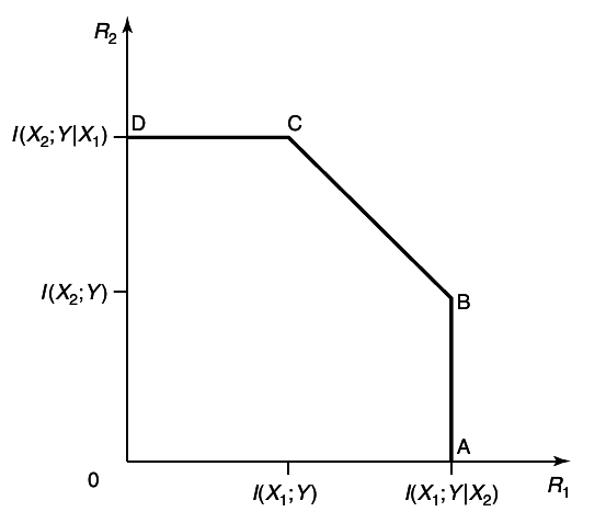
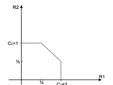
1.3.2 Comments on the Capacity Region for the Multiple-Access Channel
We have now proved the achievability of the capacity region of the multiple-access channel, which is the closure of the convex hull of the set of points (R1, R2) satisfying
for some distribution
p(x1)p(x2) on
X1 xX2. For a particular
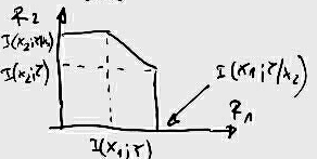
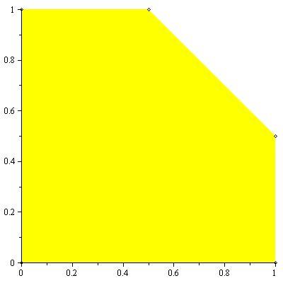
p(x1)p(x2) the region is illustrated in
17↓\begin_inset Separator latexpar\end_inset
I(X2;Y|X1) = H(X2|X1) − H(X2|X1Y) = H(X2) − H(X2|X1Y) ≥ H(X2) − H(X2|Y) = I(X2;Y);
\mathchoiceI(X2;Y|X1) ≥ I(X2;Y)I(X2;Y|X1) ≥ I(X2;Y)I(X2;Y|X1) ≥ I(X2;Y)I(X2;Y|X1) ≥ I(X2;Y)
\mathchoice\overset(a)I(X2;Y|X1) + \overset(b)I(X1;Y) = I(X1X2;Y)\overset(a)I(X2;Y|X1) + \overset(b)I(X1;Y) = I(X1X2;Y)\overset(a)I(X2;Y|X1) + \overset(b)I(X1;Y) = I(X1X2;Y)\overset(a)I(X2;Y|X1) + \overset(b)I(X1;Y) = I(X1X2;Y)
(a) - максимална брзина што може да ја постигне предавателот 2
(b)- максимална брзина што може да ја постигне предавателот 1, а притоа предавателот 2 пренесува со максиламанта брзина
Оттука произлегува дека вкупната брзина е R = R1 + R2 < I(X1X2;Y).
Let us now interpret the corner points in the region.
Point A corresponds to the maximum rate achievable form sender 1 to receiver when sender 2 is not sending any information. This is
Now for any distribution p1(x1)p2(x2),
Логично е неравенството зошто сумата претставува средна вредност, а средната вредност е секогаш помала од максималната вредност.
since the average is less than the maximum.
Therefore, the maximum in 44↑ is attained when we set X2 = x2, where x2 is the value that maximizes conditional mutual information between X1 and Y. The distribution of
X1 is chosen to maximize this mutual information. Thus,
X2 must facilitate the transmission of
X1 by setting
X2 = x2.
The point B corresponds to the maximum rate at which sender 2 can send as long as sender 1 sends at his maximum rate. This is the rate that is obtained if X1 is considered as noise for the channel from X2 to Y
Види го примерот со 15.3.3 многу јасно е објаснато ова!!!
. In this case using the results form single-user channels,
X2 can send at a rate
I(X2;Y). The receiver now knows which
X2 code-word was used and can „subtract” its effect form the channel. We can consider the channel now to be an indexed set of single-user channels, where the index is the
X2 symbol used. The
X1 rate achieved in this case is the average mutual information where the average is over these channels, and each channel occurs as many times as the corresponding
X2 symbol appears in the codewords
Многу ефективно објаснувње!!!
. Hence, the rate achieved is
Points C and D correspond to B and A respectively, with the role of the senders reversed. The non-corner points can be achieved by time-sharing. Thus, we have given a single-user interpretation and justification for the capacity region of a multiple-access channel.
The idea of considering other signals as part of the noise, decoding one signal, and then „subtracting” it form the received signal is a very useful one. We will come across the same concept again in the capacity calculations for the degraded broadcast channel.
1.3.3 Convexity of the Capacity Region of the Multiple - Access Channel
We now recast the capacity region of the multiple-access channel in order to take into account the operation of taking the convex hull by introducing a new random variable. We begin by proving that the capacity region is convex.
The capacity region C of a multiple-access channel is convex [i.e., if (R1, R2) ∈ C and (R1’, R2’) ∈ C ,then (λR1 + + (1 − λ)R1’, λR2 + (1 − λ)R2’) ∈ C for 0 ≤ λ ≤ 1].
Откако го поминав доказот на Theorem 15.3.4 ова би го парафразирал вака: Convex combination of achievable rates is achievable!
The idea is time-sharing. Given two sequences for codes at different rates R = (R1R2) and R’ = (R1’, R2’), we can construct a third codebook at rate λR + (1 − λ)R’ by using the first codebook for the first λn symbols and using the second codebook for the last (1 − λ)n symbols. The number of X1 codewords in the new code is
and hence the rate of the new code is λR + (1 − λ)R’ . Since the overall probability of error is less than the sum of the probabilities of error for each of the segments, the probability of error of the new code goes to 0 and the rate is achievable.
We can now recast the statement of the capacity region for the multiple access channel using a time-sharing random variable Q. Before we prove this result, we need to prove a property of convex sets defined by linear inequalities like those of the capacity region of the multiple-access channel.
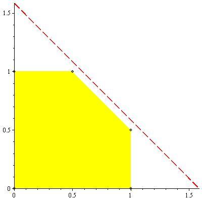
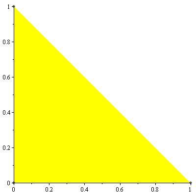
In particular, we would like to show that the convex hull of two such regions defined by linear constraints is the region defined by the convex combination of the constraints. Initially, the equality of these two sets seems obvious, but on closer examination, there is a subtle difficulty due to the fact that some of the constraints might not be acti+ve. This is best illustrated by an example. Consider the following two sets defined by linear inequalities:
In this case, the ⎛⎝(1)/(2), (1)/(2)⎞⎠ convex combination of the constraints defines the region
It is not difficult to see that any point in C1 or C2 has x + y < 20, so any point in the convex hull of the union of C1 or C2 has x + y < 20, so any point in the convex hull of the union of C1 and C2 satisfies this property. Thus, the point (15, 15), which is in C, is not in the convex hull of (C1∪C2). This example also hints at the cause of the problem - in the definition for C1, the constraint x + y ≤ 100 is not active. If this constraint were replaced by constraint x + y ≤ a, where a ≤ 20, the above result of the equality of the two regions would be true, as we now prove.
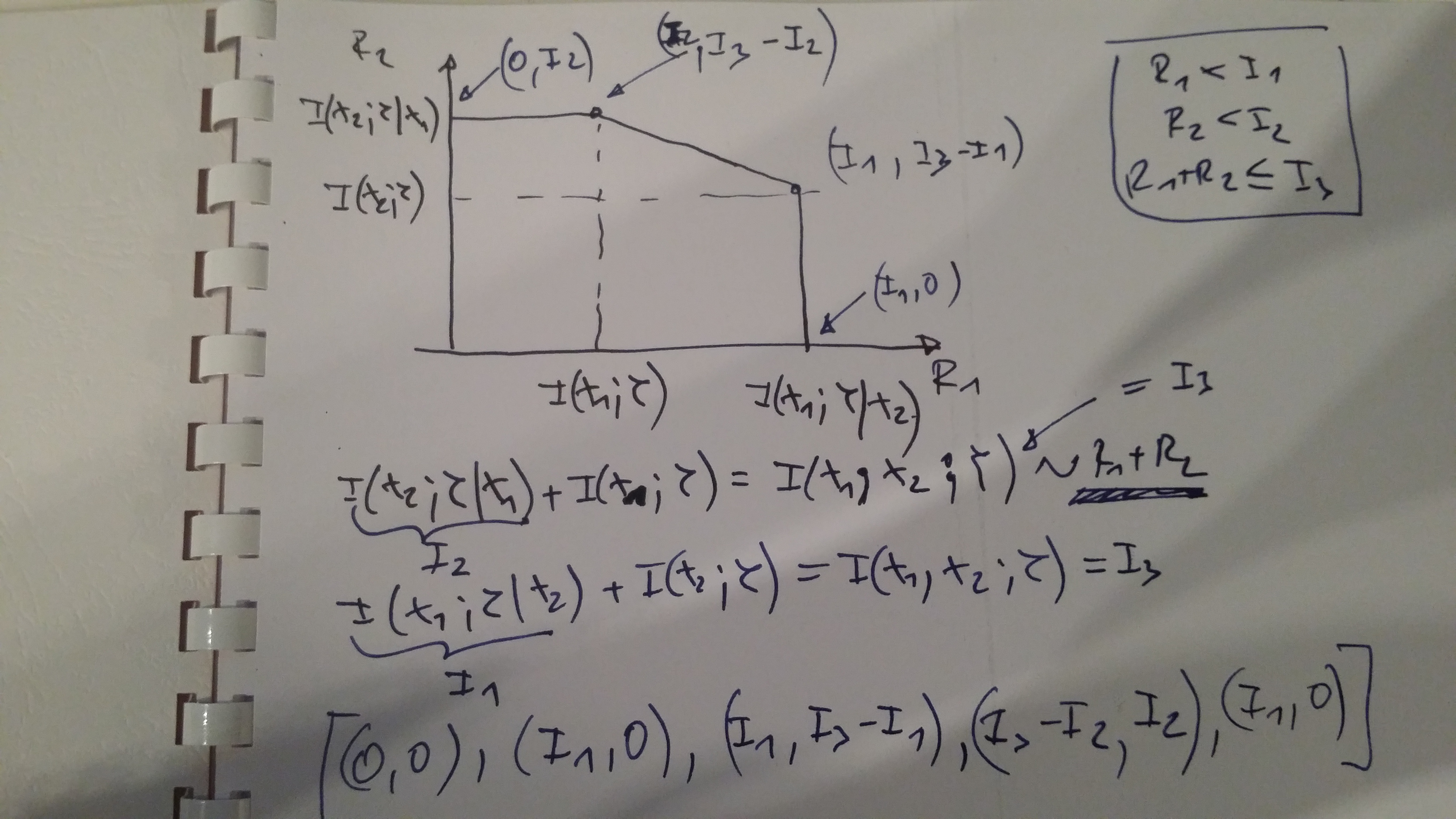
We restrict ourselves to the pentagonal regions that occur as components of the capacity region of two-user multiple-access channel. In this case, the capacity region for a fixed p(x1)p(x2) is defined by three mutual informations, I(X1;Y|X2), I(X2;Y|X1) and I(X1, X2;Y), which we shall call I1, I2 and I3, respectively. For each p(x1)p(x2) , there is a corresponding vector, I = (I1, I2, I3), and a rate region defined by
Also, since for any distribution p(x1)p(x2), we have
\mathchoiceI(X2;Y|X1)I(X2;Y|X1)I(X2;Y|X1)I(X2;Y|X1) = H(X2|X1) − H(X2|Y, X1) = H(X2) − H(X2|Y, X1) = I(X2;Y, X1) = I(X2;Y) + I(X2;X1|Y)\mathchoice ≥ I(X2;Y) ≥ I(X2;Y) ≥ I(X2;Y) ≥ I(X2;Y)
Ова истово го докажав на сличен начин во 1.3.2↑. Суштински е да имаш во предвид дека X1 и X2 се независни.
and therefore
I(X1;Y|X2) + I(X2;Y|X1) ≥ I(X1;Y|X2) + I(X2;Y) = I(X1X2;Y) → \mathchoiceI(X1;Y|X1) + I(X2;Y|X1) ≥ I(X1, X2;Y)I(X1;Y|X1) + I(X2;Y|X1) ≥ I(X1, X2;Y)I(X1;Y|X1) + I(X2;Y|X1) ≥ I(X1, X2;Y)I(X1;Y|X1) + I(X2;Y|X1) ≥ I(X1, X2;Y)
we have for all vectors I that \mathchoiceI1 + I2 ≥ I3I1 + I2 ≥ I3I1 + I2 ≥ I3I1 + I2 ≥ I3 . This property will turn out to be critical for the theorem.
Let
I1, I2 ∈ R3 be two vectors of mutual informations that define rate regions
CI1 and
CI2, respectively, as given in
51↑. For
0 ≤ λ ≤ 1 define
Iλ = λI1 + (1 − λ)I2 and let
CIλ be the rate region defined by
Iλ. Then
We shall prove this theorem in two parts. We first show that any point in the (λ, 1 − λ) mix of the sets CI1 and CI2 satisfies the inequalities for I1 and point in CI2 satisfies the inequalities for I2, so the (λ, 1 − λ) mix of these points will satisfy the (λ, 1 − λ) mix of the constraints. Thus, it follows that
To prove the reverse inclusion, we consider the extreme points of the pentagonal regions.
It is not difficult to see that the rate regions defined in 51↑ are always in the form of a pentagon, or in the extreme case when I3 = I1 + I2 in the form of a rectangle
Ова е добро илустрирано во Maple worksheet-от
. Thus, the capacity region
CI can be also defined as a convex hull of five points:
Ова многу добро го илустрирав во соодветниот Maple worksheet.
Consider the region defined by Iλ ; it, too, is defined by five points. Take any one of the points, say (I(λ)3 − I(λ)2, I(λ)2). This point can be written as the (λ, 1 − λ) mix of the points (I(1)3 − I(1)2, I(1)2) and (I(2)3 − I(2)2, I(2)2), and therefore lies in the convex mixture of CI1 and CI2. Thus, all extreme points of the pentagon CIλ lie in the convex hull of CI1 and CI2, or
Combining the two parts we have the theorem.
In the proof of the theorem, we have implicitly used the fact that all the rate regions are defined by five extreme points (at worst, some of the points are equal). all five points defined by the
I vector were within the rate region. If the condition
I3 ≤ I1 + I2 is not satisfied, some of the points in
54↑ may be outside the rate region and the proof collapses.
As an immediate consequence of the above lemma, we have the following theorem:
The convex hull of the union of the rate regions defined by individual I vectors is equal to the rate region defined by the convex hull of the I vectors.
These arguments on the equivalence of the convex hull operation on the rate regions with the convex combinations of the mutual informations can be extended to the general
m-user multiple-access channel. A proof along these lines using the theory of polymatroids is developed in
[4].
The set of achievable rates of a discrete memory-less multiple-access channel is given by the closure of the set of all (R1R2) pairs satisfying
Во ваква форма ги сведуваат во Capacity Theorem.
R1 < I(X1;Y|X2, Q) ≤ I(X1;Y|X2)
R2 < I(X2;Y|X1, Q) ≤ I(X2;Y|X1)
R1 + R2 < I(X1, X2;Y|Q) ≤ I(X1X2;Y)
Интерпретацијата е едноставна. Q e time-sharing променлива. Во генерален случај на тој начин било која условена неизвесност или заедничка информација можеш да ја претставиш како сума од поединечните условени ентропии или заеднички ентропии. Преку веројатноста p(Q) = (1)/(n) се дефинира веројатноста за пренос во „еден тајмслот” од вкупноте n. Ова некако ми оди на статистичко мултиплексирање наместо на статичко. Не ги вртиш сите трансмисии по реден број туку оставаш веројатноста тоа да го одлучи. Може во екстремен случај сите n тајмслоти да ги зафати еден предевател, зошто случајноста така одлучила.
for some choice of the joint distribution \mathchoicep(q)p(x1|q)p(x2|q)p(y|x1x2)p(q)p(x1|q)p(x2|q)p(y|x1x2)p(q)p(x1|q)p(x2|q)p(y|x1x2)p(q)p(x1|q)p(x2|q)p(y|x1x2) with |Q| ≤ 4 .
We will show that every rate pair lying in the region defined in
56↑ is achievable (i.e., it lies in the convex closure of the rate pairs satisfying Theorem 15.3.1). We also show that every point in the convex closure of the region in Theorem 15.3.1 is also in the region defined in
56↑.
Consider a rate point
R satisfying the inequalities
56↑ of the theorem. We can rewrite the right-hand side of the first inequality as
where m is the cardinality of the support set of Q. We can expand the other mutual informations similarly.
For simplicity in notation we consider a rate pair as a vector and denote a pair satisfying the inequalities in
56↑ for a specific input product distribution
p1q(x1)p2q(x2) as
Rp1p2 as
Rq. Specifically, let
Rq = (R1q, R2q) be a rate pair satisfying
Then by Theorem 15.3.1.,
Rq = (R1q, R2q) is achievable. Then since
R satisfies
56↑ and we can expand the right-hand sides as in
58↑, there exists a
set of pairs Rq satisfying
61↑ such that
Ова го разбирам како проширување на 52↑ CIλ = λCI1 + (1 − λ)CI2
Since a convex combination of achievable rates is achievable, so is R. Hence, we have proven the achievability of the region in the theorem.
The same argument can be used to show that every point in the convex closure of the region in
33↑ can be written as the mixture of points satisfying
61↑ and hence can be written in the form
56↑.
The converse is proved in the next section.
The converse shows that all achievable rate pairs are of the form 56↑ and hence establishes that this is the capacity region of the multiple-access channel. The cardinality bound on the
time-sharing random variable Q is a consequence of Caratheodory’s theorem on convex sets. See discussion below.
The proof of the convexity of the capacity region shows that any convex combination of achievable rate pairs is also achievable.
We can continue this process, taking convex combinations of more points.
Мене одма ми заличи на ова изразот 62↑
Do we need to use an arbitrary number of points? Will the capacity region be increased? The following theorems says no.
Theorem 15.3.5 (Caratheodory) (MMV)
Any point in the convex closure of a compact set A in a d-dimensional euclidean space can be represented as a convex combination of d + 1 or fewer points in the original set A.
Формулатцијата на оваа теорема во книгата Convex Polytopes е:
If A is subset of Rd then every x ∈ conv(A)
conv(A) значи дека x e точка од convex hull од A
is expressible in the form:
x = ∑di = 0αixi where xi ∈ A, ai ≥ 0 and ∑di = 0αi = 1
The proof may be found in Eggleston
[5] and Grunbaum
[6].
This theorem allows us to restrict attention to a certain finite convex combination when calculating the capacity region. This is an important property because without it, we would not be able to compute the capacity region in
56↑, since we would never know whether using a larger alphabet
Q would increase the region.
In the multiple-access channel, the bounds define a connected compact set in three dimensions. Therefore, all points in its closure can be defined as the convex combination of at most four points. Hence, we can restrict the cardinality of Q to at most 4 in the above definition of the capacity region.
Many of the cardinality bounds may be slightly improved by introducing other considerations. For example, if we are only interested in the boundary of the convex hull of A as we are in capacity theorems, a point on the boundary can be expressed as a mixture of d points of A, since a point on the boundary lies in the intersection of A with a (d − 1) - dimensional support hyperplane.
1.3.4 Converse for the Multiple-Access Channel
We have so far proved the achievability of the capacity region. In this section we prove the converse.
Proof: (Converse to Theorems 15.3.1 and 15.3.4)
We must show that given any sequence of \mathchoice((2nR1, 2nR2), n)((2nR1, 2nR2), n)((2nR1, 2nR2), n)((2nR1, 2nR2), n) codes with P(n)e → 0 the rates must satisfy
for some choice of random variable Q defined on {1, 2, 3, 4} and joint distribution p(q)p(x1|q)p(x2|q)p(y|x1x2). Fix n. Consider the given code of block length n. The joint distribution on W1 xW2 xXn1 xXn2 xYn is well defined. The only randomness is due to the random uniform choice of indices W1 and W2 and the randomness induced by the channel. The joint distribution is
where p(xn1|w1) is either 1 or 0, depending on whether xn1 = x1(w1), the codeword corresponding to w1, or not, and similarly, p(xn2|w2) = 1 or 0, according to whether xn2 = x2(w2) or not. The mutual informations that follow are calculated with respect to this distribution.
By the code construction, it is possible to estimate (W1, W2) from the received sequence Yn with low probability of error. Hence, the conditional entropy of (W1W2) given Yn must be small. By Fano’s inequality,
H(W1, W2|Yn) ≤ n(R1 + R2)P(n)e + H(P(n)e)≜nϵn
It is clear that ϵn → 0 as P(n)e. Then we have
We can now bound the rate R1 as
= H(Xn1(W1)) − H(X(n)1(W1)|Yn)\overset(c) ≤ \mathchoiceH(X(n)1(W1)|X(n)2(W2)) − H(X(n)1(W1)|Yn, X(n)2(W2)) + nϵnH(X(n)1(W1)|X(n)2(W2)) − H(X(n)1(W1)|Yn, X(n)2(W2)) + nϵnH(X(n)1(W1)|X(n)2(W2)) − H(X(n)1(W1)|Yn, X(n)2(W2)) + nϵnH(X(n)1(W1)|X(n)2(W2)) − H(X(n)1(W1)|Yn, X(n)2(W2)) + nϵn =
= I(X(n)1(W1);Yn|X2(W2)) + nϵn = H(Y(n)|Xn2(W2)) − H(Yn|X(n)2(W2), X(n)1(W1)) + nϵn =
\overset(d) = H(Yn|Xn2(W2)) − n⎲⎳i = 1H(Yi|Yi − 1Xn2(W2), X(n)1(W1)) + nϵn =
\overset(e) = H(Yn|X(n)2(W2)) − n⎲⎳i = 1H(Yi|X1i, X2i) + nϵn\overset(f) ≤ n⎲⎳i = 1H(Yi|Xn2(W2)) − n⎲⎳i = 1H(Yi|X1i, X2i) + nϵn ≤
where
(a) follows from Fanno inequality
Веројатно на аспектот од фано дека H(W1|Yn) е многу мало.
(b) follows data-processing inequality
(c) follows from the fact that since W1 and W2 are independent, so are X(n)1(W1) and X(n)2(W2), and hence H(Xn1(W1)) = H(X(n)1(W1)|X(n)2(W2)) and H(Yn|X(n)2(W2), X(n)1(W1)) ≤ H(Yn|X(n)2(W2)) by conditioning.
(d) follows from the chain rule
(e) follows form the fact that Yi depends only on X1i and X2i by the memoryless property of the channel
(f) follows from the chain rule and removing conditioning
(g) follows from removing conditioning
Hence, we have
Similarly, we have
To bound the sum of the rates, we have
where
(a) follows from Fano’s inequality
(b) follows form the data-processing inequality
(c) follows form the chain rule
(d) follows form the fact that Yi depends only on X1i and X2i and is conditionally independent of everything else
(e) follows form the chain rule and removing conditioning
Hence we have
Овој доказ секогаш најмногу ми кажува и ме учи. Логично е се ова ако се има во предвид дека бројот на елементи во (W1W2) e 2nR1⋅2nR2. Максималната ентропија е
log(2nR1⋅2nR2) = n(R1 + R2). Од овој иницијален резултат со помош на изведувањата од
71↑ до
74↑ одма доаѓаш до резултатот во
75↑. Оригинален е начинот на добивање на изразот
69↑ и тоа делот означен во зелено т.е.
(c).
The expressions in
69↑,
70↑ and
75↑ are the averages of the mutual informaitons calculated at the empirical distributions in column
i of the codebook. We can rewrite these equations with the new variable
Q, where
Q = {1, 2, ..., n} with probability
(1)/(n). The equations become
R1 ≤ (1)/(n)n⎲⎳i = 1I(X1i;Yi|X2i) + ϵn
= (1)/(n)n⎲⎳i = 1I(X1q;Yq|X2q, Q = i) + ϵn
(1)/(n)∑ni = 1I(X1q;Yq|Q = i)
I(X1Q;YQ|Q) = H(X1Q|Q) − H(X1Q|Q, YQ)
H(X1Q|Q) = (1)/(n)∑nq = 1H(X1q|Xq − 11q) = |independence of X1qfrom Xq − 11| = (1)/(n)⋅∑nq = 1H(X1q|q)
Всушност мислам дека генијално се ослободува од сумата со користење на помошната променлива. Ама секако и без неа може да се ослободи од сумата заради независнота на X1 и X2.
24.06.2013
Во чланакот Capacity Theorem одат ушт еден чекор понатаму
R1 ≤ I(X1;Y|X2, Q) + ϵn ≤ I(X1;Y|X2) + ϵn
where X1≜X1Q, X2≜X2Q and Y≜YQ are new random variables whose distributions depend on Q in the same way as the distributions of X1i, X2i and Yi depend on i. Since W1 and W2 are independent, so are X1i(W1) and X2i(W2), and hence
Hence, taking the limit as n → ∞, P(n)e → 0, we have the following converse:
for some choice of joint distribution p(q)p(x1|q)p(x2|q)p(y|x1x2). As in Section 15.3.3, the region is unchanged if we limit the cardinality of Q to 4.
This completes the proof of the converse.
Thus, the achievability of the region of Theorem 15.3.1 was proved in Section 15.3.1. In Section 15.3.3 we showed that every point in region defined by
63↑ was also achievable.
In the converse, we showed that the region in 63↑ was best we can do, establishing that this is indeed the capacity region of the channel. Thus, the region in
33↑ cannot be any larger than the region in
63↑, and this is the capacity region of the multiple-access channel.
Во Capacity Theorem чланакот продолжуваат понатаму за релеен канал и го сведуваат на следнава форма
R1 < I(X1;Y|X2, Q) ≤ I(X1;Y|X2)
R2 < I(X2;Y|X1, Q) ≤ I(X2;Y|X1)
R1 + R2 < I(X1, X2;Y|Q) ≤ I(X1X2;Y)
Ова дефинитивно фали да се додаде и во книгата.
1.3.5 m-User Multiple-Access Channels
We will now generalize the result derived for two senders to
m senders,
m ≥ 2. The multiple-access channel in this case is shown in
19↓.
We send independent indices w1, w2, ..., wm over the channel form the senders 1, 2, ..., m respectively. The codes, rates, and achievability are all defined in exactly the same way as in the tow-sender case.
Let S ⊂ {1, 2, ..., m} , respectively. Let Sc denote the complement of S. Let R(S) = ∑i ∈ SRi and let X(S) = {Xi:i ∈ S}. Then we have the following theorem.
The capacity region of the m-user multiple-access channel is the closure of the convex hull of the rate vectors satisfying
for some product distribution p1(x1)p2(x2)...pm(xm) .
The proof contains no new ideas. There arе now 2m − 1 terms in the probability of error in the achievability proof and equal number of inequalities in the proof of the converse.
In general, the region in
78↑ is a beveled box.
1.3.6 Gaussian Multiple-Access Channels (MMV)
We now discuss the Gaussian multiple-access channel of Section 15.1.2. in somewhat more detail.
Two senders, X1 and X2, communicate to the single receiver, Y. The received signal at time i is:
where
{Zi} is sequence of independent, identically distributed, zero-mean Gaussian random variables with variance
N 20↓
We assume that there is a power constraint Pj on sender j; that is, for each sender for all messages we must have
Just as the proof of achievability of channel capacity for the discrete case (Chapter 7) was extended to the Gaussian channel (Chapter 9) we can extend the proof for the discrete multiple-access channel to the Gaussian multiple-access channel. The converse can also be extended similarly, so we expect the capacity region to be the convex hull of the set of rate pairs satisfying
for some input distribution f1(x1)f2(x2) satisfying EX21 ≤ P1 and EX22 ≤ P2.
Now we can expand the mutual information in terms of relative entropy, and thus
\mathchoiceI(X1;Y|X2) = h(Y|X2) − h(Y|X1X2) = h(X1 + X2 + Z|X2) − h(X1 + X2 + Z|X1X2) = I(X1;Y|X2) = h(Y|X2) − h(Y|X1X2) = h(X1 + X2 + Z|X2) − h(X1 + X2 + Z|X1X2) = I(X1;Y|X2) = h(Y|X2) − h(Y|X1X2) = h(X1 + X2 + Z|X2) − h(X1 + X2 + Z|X1X2) = I(X1;Y|X2) = h(Y|X2) − h(Y|X1X2) = h(X1 + X2 + Z|X2) − h(X1 + X2 + Z|X1X2) =
(a) - follows from the fact that
Z is independent of
X1 an
X2, and (b) from the fact that normal maximizes entropy for a given second moment. Thus, the maximizing distribution is
X1 ~ N(0, P1) and
X2 ~ N(0, P2) with
X1 and
X2 independent. This distribution simultaneously maximizes the mutual information bounds in
81↑-
83↑.
We define the channel capacity function
corresponding to the channel capacity of Gaussian white-noise channel with signal-to-noise ratio
x (
21↓). Then we write the bound on
R1 as
and
(1)/(2)⋅log⎛⎝(N + P1)/(N)⎞⎠ + (1)/(2)⋅log⎛⎝(N + P2)/(N)⎞⎠ = ??
I(X1;Y) = (1)/(2)⋅log(E[X21] + E[X22] + N) − (1)/(2)log(E[X22] + N)
I(X1;Y|X2) = (1)/(2)⋅log(E[X21] + N) − (1)/(2)log(N) = (1)/(2)log⎛⎝(P1 + N)/(N)⎞⎠
не може вака туку треба:
I(X1X2;Y) = H(Y) − H(Y|X1X2) = H(X1 + X2 + Z) − H(X1 + X2 + Z|X1X2) ≤ (1)/(2)log(2πe)(P1 + P2 + N) − (1)/(2)log(2πe)(N) = C⎛⎝(P1 + P2)/(N)⎞⎠
I(X2;Y) = I(X1X2;Y) − I(X1;Y|X2) = (1)/(2)log⎛⎝(N + P1 + P2)/(N)⎞⎠ − (1)/(2)⋅log⎛⎝(N + P1)/(N)⎞⎠ = (1)/(2)log⎛⎝⎛⎝(N + P1 + P2)/(\cancelN)⎞⎠⎛⎝(\cancelN)/(N + P1)⎞⎠⎞⎠ = (1)/(2)log⎛⎝(N + P1 + P2)/(N + P1)⎞⎠ = (1)/(2)log⎛⎝1 + (P2)/(N + P1)⎞⎠ = C⎛⎝(P2)/(N + P1)⎞⎠
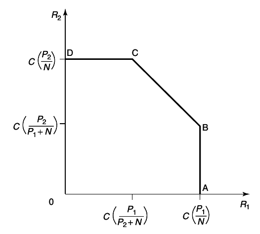
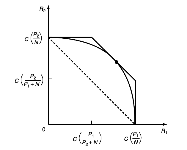
These upper bounds are achieved when X1 ~ N(0, P1) and X2 = N(0, P2) and define the capacity region. The surprising fact about these inequalities is that the sum of the rates can be as large as C⎛⎝(P1 + P2)/(N)⎞⎠ which is the rate achieved by a single transmitter sending with a power equal to the sum of the powers.
The interpretation of the corner points is very similar to the interpretation of the achievable rate pairs for a discrete multiple-access channel for a fixed input distribution. In the case of the Gaussian channel, we can consider decoding as a two-stage process:
In the fist stage, the receiver decodes the second sender, considering the first sender as part of the noise. This decoding will have low probability of error if R2 < C⎛⎝(P2)/(P1 + N)⎞⎠.
After the second sender has been decoded successfully, it can be subtracted out and the first sender can be decoded correctly if R1 ≤ C⎛⎝(P1)/(N)⎞⎠. Hence, this argument shows that we can achieve the rate pairs at the corner points of the capacity region by means of single-user operations. This process called
onion-peeling, can be extended to any number of users.
Види го завршетокот на оваа глава.
Суштината на onion-peeling е постапката каде еден сигнал се декодира, а сите други (недекодирани до тогаш) се сметаат за шум. Декодираниот сигнал се одзема од резултантниот и се продолжува со декодирање на преостанатите сигнали.
If we generalize this to
m senders with equal power, the total rate is
C⎛⎝(mP)/(N)⎞⎠ which goes to
∞ as
m → ∞ .
The average rate per sender (1)/(m)⋅C⎛⎝(mP)/(N)⎞⎠ goes to 0. Thus, when the total number of senders is very large, so that there is a lot of interference,
we can still send a total amount of information that is arbitrarily large even though the rate per individual sender goes to 0.
The capacity region described above corresponds to code-division multiple access CDMA, where separate codes are used for the different senders and the receiver decodes them one by one. In many practical situations, though, simpler schemes, such as frequency-division multiplexing or time-division multiplexing, are used. With frequency-division multiplexing, the rates depend on the bandwidth allotted to each sender. Consider the case of two senders with powers P1 and P2 using non-intersecting frequency bands with bandwidths W1 and W2, where W1 + W2 = W (Total bandwidth). Using the formula for the capacity of a single-user band-limited channel, the following rate pair is achievable:
As we vary
W1 and
W2, we trace out the curve as shown in
23↓.
This curve touches the boundary of the capacity region at one point, which corresponds to allotting bandwidth to each channel proportional to the power in that channel. We conclude that no allocation of frequency bands to radio stations can be optimal unless the allocated powers are proportional to the bandwidths.
In time-division multiple access (TDMA), time is divided into slots, and each user is allotted a slot during which only that user will transmit and every other user remains quiet. If there are two users, each of power P, rate that each sends when the other is silent is C(P ⁄ N) . Now if time is divided into equal-length slots, and every odd slot is allocated to user 1 and every even slot to user 2, the average rate that each user achieves is (1)/(2)C(P ⁄ N) . This system is called naive time-division multiple access (TDMA). However it is possible to do better if we notice that since user 1 is sending only half the time, it is possible for him to use twice the power during his transmissions and still maintain the same average power constraint. With this modification, it is possible for each user to send information at a rate (1)/(2)C(2P ⁄ N). By varying the lengths of the slots allotted to each sender (and the instantaneous power used during the slot), we can achieve the same capacity region as FDMA with different bandwidth allocations.
As
23↑ illustrates, in general the capacity region is larger than that achieved by time- or frequency-division multiplexing.
But note that the multiple-access capacity region derived above is achieved by use of a common decoder for all the senders. However, it is also possible to achieve the capacity region by onion-peeling, which removes the need for a common decoder and instead, uses a sequence of single-user codes. CDMA achieves the entire capacity region, and in addition, allows new users to be added easily without changing the codes of the current users.
On the other hand, TDMA and FDMA systems are usually designed for a fixed number of users and it is possible that either some slots are empty (if actual users is less than the number of slots) or some users are left out (if the number of users is greater than the number of slots). However, in many practical systems, simplicity of design is an important consideration, and the improvement in capacity due to the multiple-access ideas presented earlier may not be sufficient to warrant the increased complexity.
For a Gaussian multiple-access system with m sources with powers P1, P2, ..., Pm and ambient noise of power N, we can state the equivalent of Gauss’s law for аny set S in the form
1.4 Encoding of correlated sources
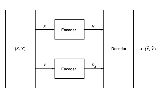
We now turn to distributed data compression. This problem is in many ways the data compression dual to the multiple-access channel problem. We know now to encode a source
X. A rate
R ≥ H(X) is sufficient. Now suppose that there are two source
(X, Y) ~ p(x, y). A rate
H(X, Y) is sufficient if we are encoding them together.
Откако го поминав проблемот 15.1 т.е. 15.2 ми стана јасна една фундаментална работа. H(X, Y)е дефиниран на множетво со следниве елементи XxY кое има |XxY| = 2nR12nR2 = 2n(R1 + R2) елементи. Затоа овде вели дека R1 + R2 ≥ H(X, Y). Си замислуваш трета променлива која ги содржи елементите од XxY кои елементи се дистрибуирани по p(X, Y).
But what if the
X and
Y sources must be described separately for some user who wishes to reconstruct both
X and
Y. It is seen that rate
R = Rx + Ry > H(X) + H(Y) is sufficient. However, in a surprising an fundamental paper by Slepian and Wolf
[7],
it is shown that a total rate R = H(X, Y) is sufficient even for separate encoding of correlated sources.
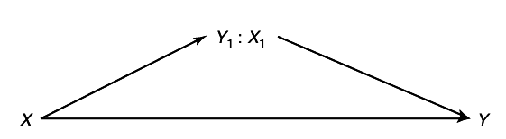
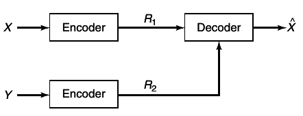
Let
(X1, Y1), (X2Y2), ... be a sequence of jointly distributed random variables i.i.d~
p(x, y). Assume that the
X sequence is available at location
A and the
Y sequence is available at a location
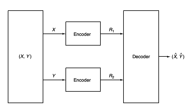
B. The situation is illustrated in
24↓.
Before we proceed to the proof of this result, we will give a few definitions.
A ((2nR1, 2nR2), n) distributed source code for the joint source (X, Y) consists of two encoder maps,
and decoder map,
g:{1, 2, ...2nR1} x{1, 2, ..., 2nR2} → XnxYn
Here f1(Xn) is the index corresponding to Xn, f2(Yn) is index corresponding to Yn, and (R1R2) is the rate pair of the code.
The probability of error for a distributed source code is defined as
A rate pair (R1R2) is said to be achievable for a distributed source if there exists a sequence of ((2nR12nR2), n) distributed source codes with probability of error P(n)e → 0. The achievable rate region is the closure of the set of achievable rates.
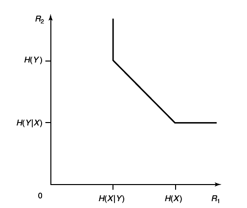
Theorem 15.4.1 (Slepian-Wolf)
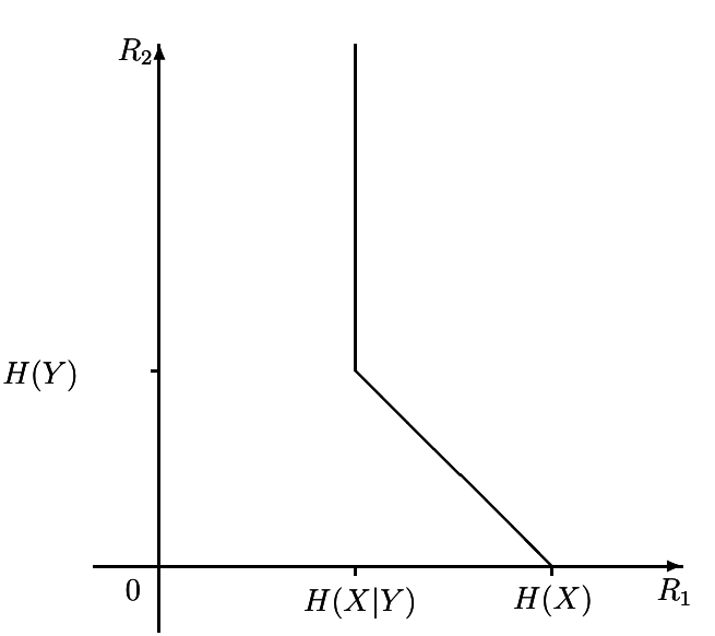
For the distributed source coding problem for the source (X, Y) drawn i.i.d ~p(x, y), the achievable rate region is given by
Значи со помалку бити можеш да го опишеш X и Y поединечно но и заедно. На пример во случај на X наместо да користиш H(X) може да користиш H(X|Y) бити (Види Source Coding with side information).
Let as illustrate the result with some examples.
Consider the weather in Gotham and Metropolis. For the purposes of our example, we assume that Gotham is sunny with probability 0.5 and that the weather in Metropolis is the same as in Gotham with probability 0.89. The joint distribution of weather is given as
X − Gotham
Y − Metropolis
X ∈ {sunny, cloudy}p(X) = ⎧⎩(1)/(2), (1)/(2)⎫⎭; Y ∈ {sunny, cloudy};
p(Y|X)
sunny
cloudy
sunny
0.89
0.11
cloudy
0.11
0.89
p(X, Y) = p(X)⋅p(Y|X);
p(X, Y)
sunny
cloudy
sunny
0.445
0.055
cloudy
0.055
0.445
Assume that we wish to transmit 100 days of weather information to the National Weather Service headquarters in Washington. We could send all the 100 bits of the weather in both places, making 200 bits in all. If we decided to compress the information independently, we would still need 100⋅H(0.5) = 100 bits of information from each place, for a total of 200 bits. If, instead, we use Slepian-Wolf encoding, we need only H(X, Y)⋅100 = 150 bits total.
Сепак овде се поставува прашање со каков код ќе можеш да ја постигнеш оваа брзина. Тука само се кажува дека тоа е минималната брзина со кој можеш да ги пренесеш информациите за времето за овие два извори.
H(Y|X) = ∑(x, y)p(x, y)log(p(y|x)) = 0.89⋅log⎛⎝(1)/(0.89)⎞⎠ + 0.11⋅log⎛⎝(1)/(0.11)⎞⎠
0.89⋅log2⎛⎝(1)/(0.89)⎞⎠ + 0.11⋅log2⎛⎝(1)/(0.11)⎞⎠ = 0.5
H(X, Y) = H(X) + H(Y|X) = 1 + 0.5 = 1.5
- Ако X и Y се независни тогаш нема спас мора да пратиш 200 бити
p(Y|X)
sunny
cloudy
sunny
0.5
0.5
cloudy
0.5
0.5
H(X, Y) = H(X) + H(Y) = 1 + 1 = 2
или
H(X, Y) = 4⋅(1)/(2)⋅log2 = 2
Мене ми е апсолутно логично корелирани извори да може да се пренесат со помала брзини од некорелирани!!!
Consider the following joint distribution
p(u, v)
0
1
0
(1)/(3)
(1)/(3)
1
0
(1)/(3)
H(U, V) = 3⋅(1)/(3)⋅log3 = 1.58
In this case, the total rate required for the transmission of this source is H(U) + H(U|V) = log3 = 1.58 bits rather than the 2 bits that would be needed if the sources were transmitted independently without Slepian-Wolf encoding.
1.4.1 Achievability of the Slepian-Wolf Theorem (random bins)
We now prove the achievability of the rates in the Slepian-Wolf theorem. Before we proceed to the proof,
we introduce a new coding procedure using random bins.
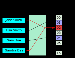
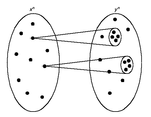
The essential idea of random bins is very similar to hash functions: We choose a large random index for each source sequence. If the set of typical source sequences is small enough (or equivalently, the range of the hash function is large enough), then with high probability, different source sequences have different indices, and we can recover the source sequence from the index.
From Wikipedia
A hash function is any function that maps data of arbitrary length to data of a fixed length. The values returned by a hash function are called hash values, hash codes, hash sums, checksums or simply hashes.
Let us consider the application of this idea to the encoding of a single source. In Chapter 3 the method that we consider was to index all elements of the typical set and not bother about elements outside the typical set. We will now describe the random binning procedure, which indexes all sequences but rejects untypical sequences at a later stage.
Consider the following procedure: For each sequence Xn, draw an index at random from {1, 2, ...2nR}. The set of sequences Xn which have the same index are said to form a bin, since this can be viewed as first laying down a row of bins and then throwing the Xn’s at random into the bins. For decoding the source frоm the bin index, we look for a typical Xn sequence in the bin. If there is one an only one typical Xn sequence in the bin, we declare it to be the estimate X̂n of the source; otherwise, an error is declared.
The above procedure defines a source code. To analyze the probability of error for this code, we will now divide the Xn sequences into two types, typical sequences and non-typical sequences. If the source sequence is typical, the bin corresponding to this source sequence will contain at least one typical sequence (the source sequence itself). Hence there will be an error only if there is more than one typical sequence in the bin. If the source sequence is non-typical, there will aways be an error. But if the number of bins is much larger than the number of typical sequences, the probability that there is more than one typical sequence in a bin is very small, and hence the probability that a typical sequence will result in an error is very small.
Formally, let f(Xn) be the bin index corresponding to Xn. Call the decoding function g. The probability of error (averaged over the random choice of code f) is:
P(g(f(X)) ≠ X) ≤ P(X ≠ A(n)ϵ) + ⎲⎳xP(∃x’ ≠ x:x’ ∈ A(n)ϵ, f(x’) = f(x))p(x)
≤ ϵ + ⎲⎳x ⎲⎳\oversetx’x’ ≠ xP(f(x’) = f(x))p(x) ≤ ϵ + ⎲⎳x ⎲⎳x’ ∈ A(n)ϵ2 − nRp(x) = ϵ + ⎲⎳x’ ∈ A(n)ϵ2 − nR ⎲⎳xp(x) ≤ ϵ + ⎲⎳x’ ∈ A(n)ϵ2 − nR ≤ ϵ + 2n(H(X) + ϵ)2 − nR ≤ 2ϵ
if \mathchoiceR > H(X) + ϵR > H(X) + ϵR > H(X) + ϵR > H(X) + ϵ and n is sufficiently large. Hence, if the rate of the code is greater that the entropy, the probability of error is arbitrarily small and the code achieves the same results as the code described in Chapter 3.
The above example illustrates the fact that there are many ways to construct codes with low probabilities of error at rates above the entropy of the source; The universal source code is another example of such a code.
Note that the binning scheme does not require an explicit characterization of the typical set at the encoder; it is needed only at the decoder. It is this property that enable this code to continue to work in the case of a distributed source, as illustrated in the proof of the theorem.
We now return to the consideration of the distributed source coding and prove the achievability of the rate region in the Slepian-Wolf theorem.
Proof: (Achievability in Theorem 15.4.1)
The basic idea of the proof is to partition the space of Xn into 2nR1 bins and the space of Yn into 2nR2 bins.
Assign every
x ∈ Xn to one of
2nR1 bins independently according uniform distribution on
{1, 2, ...2nR1}. Similarly, randomly assign every
y ∈ Yn to one of
2nR2 bins.
Reveal the assignments f1 and f2 to both the encoder and the decoder.
Sender 1 sends the index of the bin to which X belongs. Sender 2 sends the index of the bin to which Y belongs.
Given the received index pair
(i0, j0), declare
(x̂, ŷ) = (x, y) if there is one and only one pair of sequences
(x, y) such that
f1( x) = i0,
f2( y) = j0 and
(x, y) ∈ A(n)ϵ. Otherwise declare an error. The scheme is illustrated in
25↓.
The set of X sequences and the set of Y sequences are divided into bins in such a way that the pair of indices specifies a product bin.
Let (XiYi) ~ p(x, y). Define the events
E1 = {∃ x’ ≠ X:f1( x’) = f1( X) and (x’, Y) ∈ A(n)ϵ}
E2 = {∃ y’ ≠ Y:f2( y’) = f2( Y) and (X, y’) ∈ A(n)ϵ}
and
E12 = {∃( x’, y’):x’ ≠ X, y’ ≠ Y, f1( x’) = f1( X), f2( y’) = f2( Y) and (x’, y’) ∈ A(n)ϵ}
Here X, Y, f1 and f2 are random. We have an error if (X, Y) is not in A(n)ϵ or if there is another typical pair in the same bin. Hence by the union of events bound,
P(n)e = P(E0∪E1∪E2∪E12) ≤ P(E0) + P(E1) + P(E2) + P(E12)
First consider E0. By the AEP, P(E0) → 0 and hence for n sufficiently large, P(E0) ≤ ϵ. To bound P(E1), we have
P(E1) = P{∃x’ ≠ X: f1( x’) = f1( X), and (x’, Y) ∈ A(n)ϵ} = ⎲⎳(x, y)p(x, y)P{∃x’ ≠ x: f1( x’) = f1( x), and (x’, y) ∈ A(n)ϵ}
≤ ⎲⎳(x, y)p(x, y) ⎲⎳
x’ ≠ x
(x’, y) ∈ A(n)ϵ
P(f1( x’) = f1( x)) = ⎲⎳(x, y)p(x, y)⋅2 − nR1⋅|Aϵ(X|y)|\overset(a) ≤ 2 − nR12n(H(X|Y) + ϵ)
(a) - by the theorem 15.2.2.
which goes to 0 if R1 > H(X|Y). Hence for sufficiently large n, P(E1) ≤ ϵ. Similarly, for sufficiently large n, P(E2) ≤ ϵ if R2 > H(Y|X) and P(E12) ≤ ϵ if R1 + R2 > H(X, Y). Since the average probability of error is < 4ϵ, there exists at least one code (f*1, f*2, g*) with probability of error < 4ϵ. Thus, we can construct a sequence of codes with P(n)e → 0, and the proof of achievability is complete.
1.4.2 Converse for the Slepian-Wolf Theorem
The converse for the Slepian-Wolf theorem follows obviously from the results for a single source, but we will provide it for completeness.
Proof: (Converse to Theorem 15.4.1)
As usual, we begin with Fano’s inequality. Let f1, f2, g be fixed. Let \mathchoiceI0 = f1(Xn)I0 = f1(Xn)I0 = f1(Xn)I0 = f1(Xn) and \mathchoiceJ0 = f2(Yn)J0 = f2(Yn)J0 = f2(Yn)J0 = f2(Yn). Then
where ϵn → ∞ and n → ∞. Now adding conditioning, we also have
and
We can write a chain of inequalities
n(R1 + R2)\overset(a) ≥ H(I0, J0) = I(Xn, Yn;I0, J0) + H(I0J0|XnYn)\overset(b) = I(Xn, Yn;I0J0) =
= H(XnYn) − H(XnYn|I0J0)\overset(c) ≥ H(XnYn) − nϵn\overset(d) = nH(X, Y) − nϵn
where
(a) follows form the fact that I0 ∈ {1, 2, ...2nR1} and J0 ∈ {1, 2, ...2nR2}
(b) follows form the fact that I0 is a function of Xn and J0 is a function of Yn
(c) follows from the Fanno inequality
98↑.
(d) follows from the chain rule and the fact that (Xi, Yi) are i.i.d
nR1\overset(a) ≥ H(I0) ≥ H(I0|Yn) = I(Xn;I0|Yn) + H(I0|XnYn)\overset(b) = I(Xn;I0|Yn) = H(Xn|Yn) − H(Xn|I0, J0, Yn)\overset(c) ≥ H(Xn|Yn) − nϵn\overset(d) = nH(X|Y) − nϵn
J0 = f(Yn)
where the reasons are the same as for the equations above. Similarly we can show that
Dividing these inequalities by n and taking the limit as n → ∞ we have the desired converse.
The region described in the Slepian-Wolf theorem is illustrated in
27↓.
1.4.3 Slepian-Wolf Theorem for Many Sources
The results of 15.4.2 can easily be generalized to many sources. The proof follows exactly the same lines.
Let (X1i, X2i, ..., Xmi) be i.i.d ~ p(x1x2, ..., xm). Then the set of rate vectors achievable for distributed source coding with separate encoders and a common decoder is defined by
for all S ⊂ {1, 2, ..., m} where
and X(S) = {Xj:j ∈ S}.
The proof is identical to the case of two variables and is omitted.
The achievability of Slepian-Wolf encoding has been proved for an i.i.d correlated source,
but the proof can easily be extended to the case of an arbitrary joint source that satisfies the AEP; in particular, it can be extended to the case of any joint ergodic source
[8]. In these cases the entropies in the definition of the rate region are replaced by the corresponding entropy rates.
Дали постои разлика меѓу корелиран и условно зависни случајни променливи. Мислам дека нема разлика. Тогаш i.i.d correlated source е оксиморон.
1.4.4 Interpretation of Slepian-Wolf Coding
We consider an interpretation of the corner points of the rate region in Slepian-Wolf
encoding in terms of graph coloring. Consider the point with rate
R1 = H(X), R2 = H(Y|X). Using
nH(X) bits, we can encode
Xn efficiently so that the decoder can reconstruct
Xn with arbitrary low probability of error. But
how do we code Yn with nH(Y|X) bits?
H(Y|X) ≤ H(Y) due to conditioning reduces entropy. Значи со Слепиан-Вулф кодриањето се кодира Y со помалку бити.
Looking at the picture in terms of typical sets, we see that associated with every
Xn is typical „fan” of
Yn sequences that are jointly typical with the given
Xn as shown in
28↓.
If the Y encoder knows Xn, the encoder can send the index of the Yn within this typical fan. The decoder, also knowing Xn, can then construct this typical fan and hence reconstruct Yn. But the Y encoder does not know Xn. So instead of trying to determine the typical fan, he randomly colors all Yn sequences with 2nR2 colors. If the number of colors is high enough, then with high probability all the colors in a particular fan will be different and the color of the Yn sequence will uniquely define the Yn sequence within the Xn fan. If the rate R2 > H(Y|X), the number of colors is exponentially larger than the number of elements in the fan and we can show that the scheme will have an exponentially small probability of error.
1.5 Duality between slepian-wolf encoding and multiple-access channels
With multiple-access channels, we considered the problem of sending independent messages over a channel with two inputs and only one output. With Slepian-Wolf encoding, we considered the problem of sending correlated source over a noiseless channel, with a common decoder for recovery of both sources.
Тука ми текна на примерот со Gotham и Metropolis. Како ќе ги кодираш временските-услови ако користиш слепиан-Фулф кодирање и имаш само 1.5 бити на располагање.
In this section we explore the duality between the two systems.
In
29↓ two independent messages are to be sent over the channel as Xn1 and Xn2 sequences. The receiver estimates the messages from the received sequence.
In
30↑ the correlated sources are encoded as „independent” messages
i and
j. The receiver tries to estimate the source sequences from knowledge of
i and
j.
In the proof of the achievability of the capacity region for the multiple access channel, we used a random map from the set of messages to the sequences Xn1 and Xn2. In the proof for Slepian-Wolf coding, we used random map from the set of sequences Xn and Yn to set of messages. In the proof of the coding theorem for the multiple-access channel, the probability of error was bounded by
P(n)e ≤ ϵ + ⎲⎳codewordsPr(codeword jointly typical with sequence received) = ϵ + ⎲⎳2nR1 terms2 − nI1 + ⎲⎳2nR2 terms2 − nI2 + ⎲⎳2n(R1 + R2) terms2 − nI3
where ϵ is the probability the sequences are not typical, Ri are the rates corresponding to the number of codewords that can contribute to the probability of error, and Ii corresponding mutual information that corresponds to the probability that the codeword is jointly typical with the received sequence.
In the Slepian-Wolf encoding the corresponding expression for the probability of error is
P(n)e ≤ ϵ + ⎲⎳jointly typical sequencesPr(have the same codeword) = ϵ + ⎲⎳2nH1 terms2 − nR1 + ⎲⎳2nH2 terms2 − nR2 + ⎲⎳2nH3 terms2 − nR3
where again the probability that the constraints of the AEP are note satisfied is bounded by ϵ, and the other terms refer to the various ways in which another pair sequences could be jointly typical and in the same bin as the given source pair.
The duality of the multiple-access channel and correlated source encoding is now obvious. It is rather surprising that these two systems are duals of each other; one would have expected a duality between the broadcast channel and the multiple-access channel.
1.6 Broadcast channel
The broadcast channel is communication channel in which there is one sender and two or more receivers. It is illustrated in
31↓. The basic problem is to find the set of simultaneously achievable rates for communication in a broadcast channel. Before we begin the analysis, let us consider some examples.
Example 15.6.1 (TV station)
The simplest example of the broadcast channel is a radio or TV station. But this example is slightly degenerate in the sense that normally the station wants to send the same information to everybody who is tuned in; the capacity is essentially
which may be less than the capacity of the worst receiver.
But we may wish to arrange the information in such a way that the better receivers receive extra information, which produces a better picture or sound, while worst receivers continue to receive more basic information. As TV stations introduce high-definition TV (HDTV), it may be necessary to encode the information so that bad receivers will receive the regular TV signal, while good receivers will receive the extra information for the high-definition signal. The methods to accomplish this will be explained in the discussion of the broadcast channel.
Example 15.6.2 (Lecturer in classroom)
A lecturer in classroom is communicating information to the students in the class. Due to differences among the students, they receive various amounts of information. Some students receive most of the information; others receive only a little. In the ideal situation, the lecturer would be able to tailor his or her lecture in such a way that the good students receive more information and the poor students receive at least the minimum amount of information. However, a poorly prepared lecture proceeds at the pace of the weakest student. This situation is another example of a broadcast channel.
Example 15.6.3 (Orthogonal broadcast channels)
The simplest broadcast channel consist of two independent channels to the two receivers. Here we can send independent information over both channels, and we can achieve rate
R1 to receiver 1 and
R2 to the receiver 2 if
R1 < C1 and
R2 < C2 . The capacity region is the rectangle shown in the
32↓.
Ова е како independent binary symmetric channel Example 15.3.1
Example 15.6.4 (Spanish and Dutch speaker)
To illustrate the idea of superposition, we will consider a simplified example of a speaker who can speak both Spanish and Dutch. There are two listeners: One understands only Spanish and the other understands only Dutch. Assume for simplicity that the vocabulary of each language is 220 words and that the speaker speaks at rate of 1 word per second in either language. Then he can transmit 20 bits
log|X| = log(220) = 20
of information per second to receiver 1 by speaking to her all the time; in this case, he sends no information to receiver 2. Similarly, he can send 20 bits per second to receiver 2 without sending any information to receiver 1. Thus, he can achieve any rate pair with R1 + R2 = 20 by simple time-sharing. But can he do better?
Recall that the Dutch listener, even though he does not understand Spanish, can recognize when the word is Spanish. Similarly, the Spanish listener can recognize when Dutch occurs. The speaker can use this to convey information; for example, if the proportion of time he uses each language is 50%, then of a sequence of 100 words, about 50 will be Dutch and about 50 will be Spanish. But there are many ways to order the Spanish and Dutch words; in fact, there are about (10050) ≈ 2100H⎛⎝(1)/(2)⎞⎠ ways to order the words. Choosing one of these ordering conveys information to both listeners. The method enables the speaker to send information at rate of 10 bits per second to the Dutch receiver, 10 bits per second to Spanish receiver, and 1 bit per second of common information to both receivers
Од каде па сега излезе ова? Веројатно дополнителниот бит е затоа што приемникот има имплицитна информација дали е пренесен шпански или холандски збор.
, for a total rate of 21 bit per second, which is more than that achievable by simple time-sharing. This is an example of superposition of information.
The results of the broadcast channel can also be applied to the case of a single-user channel with an unknown distribution. In this case, the objective is to get at least the minimum information through when the channel is bad and to get some extra information through when the channel is good. We can use the same superposition arguments as in the case of the broadcast channel to find the rates at which we can send information.
1.6.1 Definitions for a Broadcast Channel
A broadcast channel consist of an input alphabet X and two output alphabets, Y1 and Y2, and a probability transition function p(y1, y2|x). The broadcast channel will be said to be memory-less if p(yn1, yn2|xn) = ∏ni = 1p(y1i, y2i|xi).
We define codes, probability of error, achievability, and capacity regions for the broadcast channel as we did for the multiple-access channel. A ((2nR12nR2), n) code for a broadcast channel with independent information consists of an encoder,
Ова можеш да го замислиш како една кодна листа со вкупно 2nR1 x2nR2 = 2n(R1 + R2) кодни зборови
and two decoders,
and
We define the average probability of error as the probability that the decoded message is not equal to the transmitted message; that is,
where (W1, W2) are assumed to be uniformly distributed over 2nR1 x2nR2.
A rate pair (R1R2) is said to be achievable for the broadcast channel if there exists a sequence of ((2nR1, 2nR2), n) codes with P(n)e → 0.
We will now define the rates for the case where we have common information to be sent to both receivers. A ((2nR0, 2nR1, 2nR2), n) code for broadcast channel with common information consists of an encoder
X:({1, 2, ..., 2nR0} x{1, 2, ..., 2nR1} x{1, 2, ...2nR2}) → Xn,
and two decoders,
g1: Y1 → {1, 2, ..., 2nR0} x{1, 2, ..., 2nR1}
and
g2:Y2 → {1, 2, ..., 2nR0} x{1, 2, ..., 2nR2}
We will now define the rates for the case where we have common information to be sent to both receivers
Изгледа W0 е заедничката информација што треба да се испрати.
.
Assuming that the distribution on (W0, W1, W2) is uniform, we can define the probability of error as the probability that the decoded message is not equal to the transmitted message:
λi = Pr(g(Yn) ≠ i|Xn = xn(i)) = ∑ynp(yn|xn(i))I(g(yn) ≠ i)
P(n)e = (1)/(M)∑Miλi
A rate triple (R0, R1, R2) is said to be achievable for the broadcast channel with common information if there exists a sequence of ((2nR0, 2nR1, 2nR2), n) with P(n)e → 0.
The capacity region of the broadcast channel is the closure of the set of achievable rates.
We observe that an error for receiver Yn1 depends only the distribution p(xn, yn1) and not on the joint distribution p(xn, yn1, yn2). Thus we have the following theorem:
Theorem 15.6.1 (Capacity region depends on conditional marginals)
The capacity region of a broadcast channel depends only on the conditional marginal distributions p(y1|x) and p(y2|x).
1.6.2 Degraded Broadcast Channels
Definition (physically degraded):
A broadcast channel is said to be physically degraded if \mathchoicep(y1, y2|x) = p(y1|x)⋅p(y2|y1)p(y1, y2|x) = p(y1|x)⋅p(y2|y1)p(y1, y2|x) = p(y1|x)⋅p(y2|y1)p(y1, y2|x) = p(y1|x)⋅p(y2|y1).
Definition (stochastically degraded)
A broadcast channel is said to be stochastically degraded if its conditional marginal distributions are the same as that of a physically degraded broadcast channel; that is, if there exists a distribution p’(y2|y1) such that
p(y2|x) = ⎲⎳y1p(y1|x)p’(y2|y1)
p(y1|x)⋅p(y2|y1) = p(y1|x)⋅p(y2|y1x) = p(y1y2|x) ∑y1p(y1y2|x) = p(y2|x)
Note that since the capacity of a broadcast channel depends only on the conditional marginals, the capacity region of the stochastically degraded broadcast channel is the same as that of the corresponding physically degraded channel. In much of the following, we therefore assume that the channel is physically degraded.
1.6.3 Capacity Region for the Degraded Broadcast Channel
We now consider sending independent information over a degraded broadcast channel at rate R1 to Y1 and rate R2 to Y2.
The capacity region for sending independent information over the degraded broadcast channel \mathchoiceX → Y1 → Y2X → Y1 → Y2X → Y1 → Y2X → Y1 → Y2 is the convex hull of the closure of all (R1, R2) satisfying
for some joint distribution p(u)p(x|u)p(y1, y2|x) , where the auxiliary random variable U has cardinality bounded by \mathchoice|U| ≤ min{|X|, |Y1|, |Y2|}|U| ≤ min{|X|, |Y1|, |Y2|}|U| ≤ min{|X|, |Y1|, |Y2|}|U| ≤ min{|X|, |Y1|, |Y2|}.
(The cardinality bounds for the auxiliary random variable U are derived using standard methods from convex set theory and are note dealt with here) We first give and outline of the basic idea of superposition coding for the broadcast channel. The auxiliary random variable U will serve as a cloud center that can be distinguished by both receivers Y1 and Y2. Each cloud consists of 2nR1 codewords Xn distinguishable by the receiver Y1. The worst receiver can only see the clouds, while the better receiver can see the individual codewords within the clouds. The formal proof of the achievabilty of this region uses a random coding argument:
Fix p(u) and p(x|u).
Random codebook generation:
Generate 2nR2 independent codewords of length n, U(w2), w2 ∈ {1, 2, ..., 2nR2},
Во Problem 15.11 случајната променлива Ui ја дефинираат така што зависи од втората порака и од претходните вредности на Y1
according to ∏ni = 1p(ui). For each codeword U(w2) generate 2nR1 independent codewords X(w1w2) according to ∏ni = 1p(xi|ui(w2)) . Here u(i) plays the role of the cloud center understandable to both Y1 and Y2 , while x(i, j) is the j-th satellite codeword in the i-th cloud.
Ова личи на суперпозиција на два вектори. Веројатно затоа постапкава ја вика суперпозиција.
To send the pair (W1, W2) send the corresponding codeword X(W1W2).
Receiver 2 determines the unique Ŵ̂2 such that (U(Ŵ̂2), Y2) ∈ A(n)ϵ. If there are none such or more that one such, an error is declared.
Receiver 1 looks for the unique (Ŵ1Ŵ2) such that (U(Ŵ2), X(Ŵ1Ŵ2), Y1) ∈ A(n)ϵ. If there are none such or more than one such, an error is declared.
Analysis of the probability of error:
By the symmetry of the code generation, the probability of error does not depend on which codeword was sent. Hence without loss of generality we can assume that the message pair (W1W2) = (1, 1) was sent. Let P(⋅) denote conditional probability of an event given that (1, 1) was sent.
Since we have essentially a single user channel from U to Y2, we will be able to decode the U codewords with a low probability of error if \mathchoiceR2 ≤ I(U;Y2)R2 ≤ I(U;Y2)R2 ≤ I(U;Y2)R2 ≤ I(U;Y2). To prove this we define the events
Then the probability of error at receiver 2 is:
P(n)e(2) = P(EcY1∪∪i ≠ 1EYi) ≤ P(EcY1) + ⎲⎳i ≠ 1P(EYi)\overset(a) ≤ ϵ + 2nR2⋅2 − n(I(U;Y2) − 2ϵ) ≤ 2ϵ
if n is large enough and \mathchoiceR2 < I(U;Y2)R2 < I(U;Y2)R2 < I(U;Y2)R2 < I(U;Y2) where (a) follows form AEP. Similarly, for decoding for receiver 1, we define the events
where the tilde refers to events defined at receiver 1. Then we can bound the probability of error as:
P(n)e = P(ẼcY1∪ẼcY11∪∪i ≠ 1ẼYi∪∪j ≠ 1ẼY1j) ≤ P(ẼcY1) + P(ẼcY11) + ⎲⎳i ≠ 1P(ẼYi) + ⎲⎳j ≠ 1P(ẼY1j)
Се прашувам зошто не ги зема во предвид:
⎲⎳i ≠ 1P(ẼYi1)
и
⎲⎳i ≠ 1;j ≠ 1P(ẼYij)
како на пример што прави во Multiple-access channel.
By the same arguments as for receiver 2, we can bound P(ẼYi) ≤ 2 − n(I(U;Y1) − 3ϵ) . Hence, the third term goes to 0 if
Овде e R2 затоа што i оди до 2nR2, а j оди до 2nR1
R2 < I(U;Y1). But by the data-processing inequality and the degraded nature of the channel, I(U;Y1) ≥ I(U;Y2), and hence the conditions of the theorem imply that the third term goes to 0.
\mathchoiceX → Y1 → Y2X → Y1 → Y2X → Y1 → Y2X → Y1 → Y2
p(y1, y2|x) = p(y1|x)⋅p(y2|y1)
P(X, Z|Y) = (P(X, Y, Z))/(P(Y)) = (P(X, Y)P(Z|XY))/(p(Y)) = P(X|Y)⋅P(Z|Y)
P(Y, Z|X) = (P(X, Y, Z))/(P(X)) = (P(X, Y)P(Z|XY))/(p(X)) = P(Y|X)⋅P(Z|Y)
Значи деградираност и марковитост е една иста работа!
I(U;Y1Y2) = I(U;Y1) + I(U;Y2|Y1) = I(U;Y1) + H(Y2|Y1) − H(Y2|Y1U) = I(U;Y1) =
= I(U;Y2) + \overset ≠ 0I(U;Y1|Y2) → I(U;Y1) ≥ I(U;Y2)
R2 < I(U;Y2) < I(U;Y1) ⇒ R2 < I(U;Y1)
We can also bound the fourth term in the probability of error as
P(EY1j) = P((U(1), X(1, j), Y1) ∈ A(n)ϵ) = ⎲⎳(U, X, Y1) ∈ A(n)ϵP(U(1))P(X(1, j)|U(1))P(Y1| U(1))
≤ ⎲⎳(U, X, Y1) ∈ A(n)ϵ2 − n(H(U) − ϵ)2 − n(H(X|U) − ϵ)2 − n(H(Y1|U) − ϵ)
≤ 2n(H(U, X, Y1) + ϵ)2 − n(H(U) − ϵ)2 − n(H(X|U) − ϵ)2 − n(H(Y1|U) − ϵ) = 2 − n(I(X;Y1|U) − 4ϵ)
p(U, X, Y1) = p(U)p(X|U)p(Y1|U, X1) = p(U)p(X|U)p(Y1|U)
зато што U, X, Y1 формираат марков ланец.
U → X → Y1
2n(H(U, X, Y1) + ϵ)2 − n(H(U) − ϵ)2 − n(H(X|U) − ϵ)2 − n(H(Y|U) − ϵ)
nH(U, X, Y1) + nϵ − nH(U) + nϵ − nH(X|U) + nϵ − nH(Y1|U) + nϵ = n(H(U, X, Y1) − H(U) − H(X|U) − H(Y|U) + 4ϵ)
I(X;Y1|U) = H(X|U) − H(X|U, Y1) = H(Y1|U) − H(Y1|UX)
H(U, X, Y1) − H(U) − H(X|U) − H(Y1|U) + 4ϵ =
\cancelH(U) + \cancelH(X|U) + H(Y1|X, U) − \cancelH(U) − \cancelH(X|U) − H(Y1|U) + 4ϵ = − (H(Y1|U) − H(Y1|X, U)) + 4ϵ = − I(X;Y1|U) + 4ϵ
Hence, if R1 < I(X;Y1|U),
∑j ≠ 1P(ẼY1j) ≤ 2nR12 − n(I(X;Y1|U) − 4ϵ)
the fourth term in the probability of error goes to 0. Thus we can bound the probabilities of error
P(n)e(1) ≤ ϵ + ϵ + 2nR22 − n(I(U;Y1) − 3ϵ) + 2nR12 − n(I(X;Y1|U) − 4ϵ) ≤ 4ϵ
2nR12 − n(I(X;Y1|U) − 4ϵ)
R1 < I(X;Y1|U) − 4ϵ < I(X;Y1|U) → R1 < I(X;Y1|U)
тоа не значи ако R1 < I(X;Y1|U) дека R1 < I(X;Y1|U) − 4ϵ, а обратното не важи.
if
n is large enough and
\mathchoiceR2 < I(U;Y2)R2 < I(U;Y2)R2 < I(U;Y2)R2 < I(U;Y2) and
\mathchoiceR1 < I(X;Y1|U)R1 < I(X;Y1|U)R1 < I(X;Y1|U)R1 < I(X;Y1|U). The above bounds show that we can decode the messages with total probability of error that goes to
0. Hence there exist a sequence of good
((2nR12nR2), n) codes
C*n with probability of error going to
0.
With this, we complete the proof of the achievability of capacity region for the degraded broadcast channel. Gallager’s
[9] proof of the converse is outlined in Problem 15.11.
So far we have considered sending independent information to each receiver. But in certain situations, we wish to send common information to both receivers. Let the rate at which we send common information be R0. Then we have the following obvious theorem:
If the rate pair (R1R2) is achievable for a broadcast channel with independent information, the rate triple (R0, R1 − R0, R2 − R0) with a common rate R0 is achievable, provided that R0 ≤ min(R1R2).
In this case of a degraded broadcast channel, we can do even better. Since by our coding scheme the better receiver aways decodes all the information that is sent to the worst receiver, one need not reduce the amount of information sent to the better receiver when we have common information.
If the rate pair (R1R2) is achievable for a degraded broadcast channel, the rate triple (R0, R1, R2 − R0) is achievable for the channel with common information, provided that R0 < R2.
We end this section by considering the example of the binary symmetric broadcast channel.
Consider a pair of binary symmetric channels with parameters
p1 and
p2 that form a broadcast channel as shown in
34↓. Without loss of generality in the capacity calculation, we can recast this channel as a physically degraded channel. We assume that
p1 < p2 < (1)/(2) . Then we can express a binary symmetric channel with parameter
p2 as a cascade of a binary symmetric channel with parameter
p1 with another binary symmetric channel. Let the crossover probability of the new channel be
α. Then we must have
p1(1 − α) + (1 − p1)α = p2
or
We now consider the auxiliary random variable in the definition of the capacity region. In this case cardinality of U
|U| ≤ min{|X|, |Y1|, |Y2|}
is binary from the bound of the theorem. By symmetry, we connect U to X by another binary symmetric channel with parameter β, as illustrated in
We can now calculate the rates in the capacity region. It is clear by symmetry that the distribution on U that maximizes the rates is the uniform distribution on {0, 1}, so that
R2 ≤ I(U;Y2) = H(Y2) − H(Y2|U) = 1 − H(βp2)
После проблем 15.13 ми текна дека може вакво неравенство да се напише:
R2 ≤ I(U;Y2) ≤ I(X;Y2) = H(Y2) − H(Y2|X) = 1 − H(p2)
where
Similarly,
R1 ≤ I(X;Y1|U) = H(Y1|U) − H(Y1|X, U) = H(Y1|U) − H(Y1|X) = H(βp1) − H(p1)
where
Plotting these points as function of
β, we obtain the capacity region in
1↑. When
β = 0, we have maximum information transfer to
Y2 (i.e.
R2 = 1 − H(p2) and
R1 = 0). When
β = (1)/(2), we have maximum information transfer to
Y1 (i.e.
R1 = 1 − H(p1) and no information transfer to
Y2. This values of
β give us the corner points of the rate region.
β = (1)/(2)
R1 ≤ I(X;Y1|U) = H(Y1|U) − H(Y1|X, U) = H(Y1|U) − H(Y1|X) = H(βp1) − H(p1)
βp1 = β(1 − p1) + (1 − β)p1
βp1 = (1)/(2) − (p1)/(2) + (1)/(2)p1 = (1)/(2)
R1 = H⎛⎝(1)/(2)⎞⎠ − H(p1) = 1 − H(p1)
Example 15.6.6 (Gaussian broadcast channel)
The Gaussian broadcast channel is illustrated in
37↑. We have shown it in the case where one output is a degraded version of the other output. Based on the results of Problem 15.10, it follows that all scalar Gaussian broadcast channels are equivalent to this type of degraded channel.
where Z1 ~ N(0, N1) and Z2’ ~ N(0, N2 − N1)
Extending the results of this section to the Gaussian case, we can show that the capacity region of this channel is given by:
where α may be arbitrary chosen (0 ≤ α ≤ 1). The coding scheme that achieves this capacity region is outlined in Section 15.1.3.
1.7 Relay Channel
The relay channel is a channel in which there is one sender and one receiver with a number of intermediate nodes that act as relays to help the communication form the sender to the receiver. The simplest relay channle ha only one intermediate or relay node. In this calse the channel consists of foru finite sets
X, X1, Y, and Y1 and collection of probability mass functions
p(y, y1|x, x1) on
YxY1, one for each
(x, x1) ∈ XxX1. The interpretation is that
x is the input to the channel and
y is the output of the channel,
y1 is the relay’s observation, and
x1 is the input symbol chosen by the relay, as shown in
38↓. The problem is to find the capacity of the channel between the sender
X and the receiver
Y.
The relay channel combines a broadcast channel (X to Y and Y1) and a multiple-access channel (X and X1 to Y). The capacity is known for the special case of the physically degraded relay channel. We fist prove and outer bound on the capacity of a general relay channel and later establish an achievable region for the degraded relay channel.
A (2nR, n) code for a relay channel consists of a set of integers W = {1, 2, ...2nR} , an encoding function
a set of relay functions {fi}ni = 1 such that
x1i = fi(Y11, Y12, ..., Y1i − 1) 1 ≤ i ≤ n
and decoding function
Note that the definition of the encoding functions includes the non-anticipatory condition on the relay. The relay channel input is allowed to depend only on the past observations y11, y12, ..., y1i − 1. The channel is memoryless in the sense that (Yi, Y1i) depends on the past only through the current transmitted symbols (Xi, X1i). Thus for any choice p(w), w ∈ W, and code choice X:{1, 2, ..., 2nR} → Xni and relay functions {fi}ni = 1, the joint probability mass function on WxXnxXn1 xYnxYn1 is given by:
If the message w ∈ [1, 2nR] is sent, let
λ(w) = Pr{g(Y) ≠ w|w sent }
denote the conditionla probability of error. We define the average probability of error of the code as:
The probability of error is calculated under the uniform distribution over the codewords w ∈ {1, ...2nR}. The rate R is said to be achievable by the relay channel if there exists a sequence of (2nR, n) codes with P(n)e → 0. The capacity C of a relay channel is the supremum of the set of achievable rates.
We first give and upper bound on the capacity of the relay channel.
For any relay channel (XxX1, p(y, y1|x, x1, YxY1)), the capacity C is bounded above by
The proof is direct consequence of a more general max-flow min-cut theorem given in Section 15.10.
This upper bound has a nice max-flow min-cut interpretation.
Дури сега го сконтава откако претходно го поминав max-flow min-cut алогритамот во книгата на Ford!!!
The first term in
124↑ upper bounds the maximum rate of information transfer from senders
X and
X1 to receiver
Y. The second terms bound the rate form
X to
Yand
Y1.
We now consider a family of relay channels in which the relay receiver is better then the ultimate receiver
Y in sence defined below. Here the max-flow minpcut upper bound in
124↑ is achieved.
Definition (degraded relay channel)
The relay channel (XxX1, p(y, y1|x, x1, YxY1)) is said to be physically degraded if p(y, y1|x, x1) can be written in the form
Thus, Y is random degradation of the relay signal Y1.
Broadcast channel:
p(y1, y2|x) = p(y1|x)p(y2|y1)
For the physically degraded relay channel, the capacity is given by the following theorem.
The capacity C of a physically degraded relay channel is given by:
\mathchoiceC = supp(x, x1)min{I(X, X1;Y)I(X;Y1|X1)}C = supp(x, x1)min{I(X, X1;Y)I(X;Y1|X1)}C = supp(x, x1)min{I(X, X1;Y)I(X;Y1|X1)}C = supp(x, x1)min{I(X, X1;Y)I(X;Y1|X1)}
where the supremum is over all joint distributions on XxX1.
Нека не те чуди вториот член. Од главата за multiple-access channel јасно беше дека I(X1;Y|X2) ≥ I(X1;Y)
т.е. таму е докажано следново:
\mathchoiceI(X2;Y|X1)I(X2;Y|X1)I(X2;Y|X1)I(X2;Y|X1) = H(X2|X1) − H(X2|Y, X1) = H(X2) − H(X2|Y, X1) = I(X2;Y, X1) = I(X2;Y) + I(X2;X1|Y)\mathchoice ≥ I(X2;Y) ≥ I(X2;Y) ≥ I(X2;Y) ≥ I(X2;Y)
The proof follows form theorem 15.7.1 and by degradedness since for degraded relay channel I(X;Y, Y1|X1) = I(X;Y1|X1).
p(y, y1|x, x1) = p(y1|x, x1)p(y|y1x1)
I(X;Y, Y1|X1) = I(X;Y1|X1) + I(X;Y|Y1X1) = I(X;Y1|X1) + H(X|Y1X1) − H(X|Y, Y1X1) = I(X;Y1|X1) + H(Y|Y1X1) − H(Y|X, Y1X1)
I(X;Y, Y1|X1) = H(Y, Y1|X1) − H(Y, Y1|X, X1) = H(Y, Y1|X1) − H(Y1|X, X1) − H(Y|Y1, X1) =
H(Y1|X1) + \cancelH(Y|X1Y1) − H(Y1|X, X1) − \cancelH(Y|Y1, X1) = I(X;Y1|X1)
Слично ја имам докажано во Capacity Theorem notebook-от. Таму дополнително сум замислил дека деградиреноста може да се опише со следниов марков ланец
X1 → (X2, Y1) → Y
The proof of achievable involves a combination of the following basic techniques: (1) random coding, (2) list codes, (3) Slepian-Wolf partitioning, (4) coding for te cooperative multiple access channel, (5) superposition coding, and (6) block Markov encoding at the relay and transmitter. We provide only an outline of the proof.
Outline of Achievability:
We consider B blocks of transmission, each of n symbols. A sequence of B − 1 indices, wi ∈ {1, ...2nR}, i = 1, 2, ..., B − 1, will be sent over the channel in nB transmissions. (Note that as B → ∞ for a fixed n, the rate R(B − 1) ⁄ B is arbitrarily close to R.)
We define a doubly indexed set of codewords:
We will also need a partition
S = {S1, S2, ..., S2nR0} of W = {1, 2, ..., 2nR}
into
2nR0 cells, with
Si∩Sj = ∅, i ≠ j, and ∪Si = W. The partition will enable us to send side information to the receiver in the manner of Slepian and Wolf
[7].
Generation of random code:
Fix p(x1)p(x|x1).
First generate at random 2nR0 i.i.d n- sequences in Xn1, each draw according to p(x1) = ∏ni = 1p(x1i) . Index them as x1(s), s ∈ {1, 2, ..2nR0}. For each x1(s) generate 2nR conditionally independent n-sequences x(w|s) , w ∈ {1, 2, ...2nR}, drawn independently according to p(x|x1(s)) = ∏ni = 1p(xi|x1i(s)). This defines the random codebook C = {x(w|s), x1(s)}.
Ако x1 е вектор x е дводимензионална матрица
The random partitions S = {S1, S2, ..., S2nR0} of {1, 2, ...2nR} is defined as follows. Let each integer w ∈ {1, 2, ...2nR} be assigned independently according to a uniformly distribution over the indices s = 1, 2, ...2nR0, to cells Ss.
Let wi ∈ {1, 2, ..., 2nR} be the new index to be sent in block i, and let si be as the partition corresponding to wi − 1 (i.e., wi − 1 ∈ Ssi). The encoder sends x(wi|si). The relay has an estimate ŵ̂i − 1 of the previous index wi − 1. (This will be made precise in the decoding section.) Assume that ŵ̂i − 1 ∈ Ssî̂. The relay encoder sends x1(sî̂) in block i.
We assume that at the end of block i − 1, the receiver knows (w1, w2, ...wi − 2) and (s1, s2, ..., si − 1) and the relay knows (w1, w2, ..., wi − 1) and consequently (s1, s2, ..., si). The decoding procedures at the end of block i are as follows:
1. Knowing si and upon receiving y1(i), the relay receiver estimates the message of the transmitter ŵ̂i = w if and only if there exists a unique w such that (x(w|si), x1(si), y1(i)) are jointly ϵ-typical. Using Theorem 15.2.3 it can be shown that wî̂ = wi with an arbitrarily small probability of error if
and n is sufficiently large.
2. The receiver declares that sî = s was sent iff there exists one and only one s such that (x1(s), y(i)) are jointly ϵ-typical. From Theorem 15.2.1 we know that si can be decoded with arbitrarily small probability of error if
and n is sufficiently large.
3. Assuming that si is decoded correctly at the receiver, the receiver constructs a list ℒ(y(i − 1)) of indices that the receiver considers to be jointly typical with y(i − 1) in the (i − 1)-th block. The receiver then declares ŵi − 1 = w as the index sent in block i − 1 if there is a unique w in SSi∩ℒ(y(i − 1)). If n is sufficiently large and if
then
ŵi − 1 = wi − 1 with arbitrarily small probability of error. Combining two constraints
127↑ and
128↑,
R0 drops out leaving
R < I(X;Y|X1) + I(X1;Y) = I(X, X1;Y)
For a detailed analysis of the probability of error the reader is refereed to
[10].
Theorem 15.7.2
C = supp(x, x1)min{I(X, X1;Y)I(X;Y1|X1)}
can also shown to be the capacity for the following classes of relay channels:
1. Reversely degraded relay channel, that is,
обичен деградиран канал беше p(y, y1|x, x1) = p(y1|x, x1)p(y|y1x1)
p(y, y1|x, x1) = p(y|x, x1)p(y1|y, x1)
2. Relay channel with feedback
3. Deterministic relay channel,
1.8 Source coding with side information
We now consider the distributed source coding problem where two random variables X and Y are encoded separately but only X is to be recovered. We now ask how many bits R1 are required to describe X if we are allowed R2 bits to describe Y. If R2 > H(Y) , then Y can be described perfectly, and by the results of Slepian-Wolf coding, R1 = H(X|Y) bits suffice to describe X. At the other extreme, if R2 = 0, we must describe X without any help, and R1 = H(X) bits are then necessary to describe X. In general, we use R2 = I(Y;Ŷ) bits to describe an approximate version of Y.
I(Y;Ŷ) = H(Y) − H(Y|Ŷ)
This will allow us to describe X using H(X|Ŷ) in presence of side information Ŷ. The following theorem is consistent with this intuition.
Let (X, Y) ~ p(x, y). If Y is encoded at rate R2 and X is encoded at rate R1, we can recover X with an arbitrarily small probability of error if and only if
for some joint probability mass function \mathchoicep(x, y)p(u|y)p(x, y)p(u|y)p(x, y)p(u|y)p(x, y)p(u|y), where |U| ≤ |Y| + 2.
p(x, y, u) = p(xy)p(u|xy) = p(xy)p(u|y)
Од самата дефиниција здружената веројатност следи дека X, Y, U се во марков ланец.
X → Y → U
We prove this theorem in two parts. We began with the converse, in which we show that for any encoding scheme that has a small probability of error, we can find random variable U with a joint probability mass function as in the theorem.
Consider any source code for
39↓.
The source code consists of mappings fn(Xn) and gn(Yn) such that the rates of fn and gn are less than R1 and R2, respectively, and a decoding mapping hn such that:
\mathchoiceP(n)e = Pr{hn(fn(Xn), gn(Yn)) ≠ Xn} < ϵ.P(n)e = Pr{hn(fn(Xn), gn(Yn)) ≠ Xn} < ϵ.P(n)e = Pr{hn(fn(Xn), gn(Yn)) ≠ Xn} < ϵ.P(n)e = Pr{hn(fn(Xn), gn(Yn)) ≠ Xn} < ϵ.
Define new random variables \mathchoiceS = fn(Xn)S = fn(Xn)S = fn(Xn)S = fn(Xn) and \mathchoiceT = gn(Yn)T = gn(Yn)T = gn(Yn)T = gn(Yn). Then since we can recover Xn from S and T with low probability of error, we have by Fano’s inequality,
Then
Се запрашав зошто nR2 ≥ H(T)
nR2 = H(Yn) ≥ H(g(Yn)) = H(T)
(a) follows from the fact that the range of gn is {1, 2..., 2nR2}
(b) follows from the properties of the mutual information
I(Yn;T) = H(T) − H(T|Yn) ≤ H(T)
(c) follows from the chain rule and the fact that Yi is independent of Y1, ...Yi − 1 and hence I(Yi;Y1, ..., Yi − 1) = 0
I(Yi;T, Y1, ...Yi − 1) = \overset0I(Yi;Yi − 11) + I(Yi;T|Y1, ..Yi − 1) = I(Yi;T|Y1, ..Yi − 1)
(d) follows if we define \mathchoiceUi = (T, Y1, ..., Yi − 1)Ui = (T, Y1, ..., Yi − 1)Ui = (T, Y1, ..., Yi − 1)Ui = (T, Y1, ..., Yi − 1)
We also have another chain for R1
\mathchoicenR1nR1nR1nR1\overset(a) ≥ H(S)\overset(b) ≥ H(S|T) = H(S|T) + H(Xn|S, T) − H(Xn|S, T)\overset(c) ≥ H(S, Xn|T) − nϵn\overset(d) = H(Xn|T) + \canceltoH(f(Xn)|Xn) = 0H(S|XnT) − nϵn
= H(Xn|T) − nϵn\overset(e) = ∑ni = 1H(Xi|T, X1, ..., Xi − 1) − nϵn\overset(f) ≥ \mathchoice∑ni = 1H(Xi|T, Xi − 1Yi − 1)∑ni = 1H(Xi|T, Xi − 1Yi − 1)∑ni = 1H(Xi|T, Xi − 1Yi − 1)∑ni = 1H(Xi|T, Xi − 1Yi − 1) − nϵn
\overset(g) = ∑ni = 1H(Xi|T, Yi − 1) − nϵn\overset(h) = \mathchoice∑ni = 1H(Xi|Ui)∑ni = 1H(Xi|Ui)∑ni = 1H(Xi|Ui)∑ni = 1H(Xi|Ui) − nϵn,
(a) follows from the fact that the range of
S is
{1, 2, ...2nR1}
Ако се прашуваш зошто nR1 ≥ H(S):
nR2 = H(Xn) ≥ H(f(Xn)) = H(S)
(b) follows form the fact that conditioning reduces entropy
(c) follows form Fano’s inequality
H(S|T) + H(Xn|S, T) = H(S, Xn|T)
(d) follows form the chain rule and the fact that S is a function of Xn
(e) follows form the chain rule for entropy
(f) follows from the fact that conditioning reduces entropy
(g) follows from the
(subtle) fact that
Xi → (T, Yi − 1) → Xi − 1 forms a Markov chain
since Xi does not contain any information about Xi − 1 that is not there in Yi − 1 and T = gn(Yn).
Вау! Каква фундаментална дефиниција за марков чеин. Гениално!!!
На времето имам покажано дека својството на марковиот ланец што оди нанапред важи и наназад т.е.:
H(Xi|(T, Yi − 1)Xi − 1) = H(Xi|(T, Yi − 1))
(h) follows form the definition of U
Also, since Xi contains no more information about Ui than is present in Yi, it follows that \mathchoiceXi → Yi → UiXi → Yi → UiXi → Yi → UiXi → Yi → Ui forms Markov chain.
Thus we have following inequalities:
We now introduce a time-sharing random variable Q so that we can rewrite these equations as:
Now since Q is independent of YQ (The distribution of Yi does not depend on i), we have
Now XQ and YQ have the joint distribution p(x, y) in the theorem.
XQ≜X, YQ≜Y
Defining U = (UQ, Q), X = XQ and Y = YQ we have shown the existence of the random variable U such that
for any encoding scheme that has a low probability of error. Thus, the converse is proved.
Before we proceed to the proof of the achievability of this pair of rates, we will need a new lemma about strong typicality and Markov chains. Recall the definition of strong typicality for a triple of random variables X, Y and Z. A triplet of sequences xn, yn, zn is said to be ϵ-strongly typical if (Chapter 10)
In particular, this implies that (xn, yn) are jointly strongly typical and that (yn, zn) are also jointly strongly typical. But the converse is not true:
The fact that
(xn, yn) ∈ A*(n)ϵ(X, Y) and
(yn, zn) ∈ A*(n)ϵ(Y, Z) doesn’t in general imply that
(xn, yn, zn) ∈ A*(n)ϵ(X, Y, Z).
But if X → Y → Z forms Markov chain this implication is true. We state this as lemma without proof
[1] [11].
Lemma 15.8.1 (Markov Lemma)
Let (X, Y, Z) form a Markov-chain X → Y → Z [i.e., p(x, y, z) = p(x, y)p(z|y)] . If for a given (yn, zn) ∈ A*(n)ϵ(Y, Z), Xn is drawn ~∏ni = 1p(xi|yi) then Pr{(xn, yn, zn) ∈ A*(n)ϵ(X, Y, Z)} > 1 − ϵ for n sufficiently large.
\mathchoicep(x, z|y)p(x, z|y)p(x, z|y)p(x, z|y) = (p(x, y, z))/(p(y)) = \mathchoice(p(xy)p(z|xy))/(p(y))(p(xy)p(z|xy))/(p(y))(p(xy)p(z|xy))/(p(y))(p(xy)p(z|xy))/(p(y)) = p(x|y)p(z|y)
p(y)p(x, z|y) = p(xy)\canceltop(z|y)p(z|xy) → p(x, y, z) = p(x, y)⋅p(z|y)
The theorem is true from the strong law of large numbers if Xn ~ ∏ni = 1p(xi|yi, zi). The Markovity of X → Y → Z is used to show that Xn ~ p(xi|yi) is sufficient for the same conclusion.
We now outline the proof of achievability in Theorem 15.8.1
Proof: (Achievability in Theorem 15.8.1)
Fix p(u|y). Calculate p(u) = ∑yp(y)p(u|y)
Generation of code-books:
Generate 2nR2 independent codewords of length n, U(w2), w2 ∈ {1, 2, ...2nR2} according to ∏ni = 1p(ui). Randomly bin all the Xn sequences into 2nR1 bins by independently generating an index b distributed uniformly on {1, 2, ..., 2nR1} for Xn. Let B(i) denote the set of Xn sequences allotted to bin i.
The X sender sends the index i of the bin in which Xn falls. The Y sender looks for an index s such that (Yn, Un(s)) ∈ A(n)ϵ(Y, U).
Имај во предвид дека Ui = (T, Y1, ..., Yi − 1)
If there is more than one such s, it sends the least. If there is no such Un(s) in the code-book, it sends s = 1.
Постапкава многу ми личи на методата на енкодирање и декодирање во relay channel. Можеби може да се каже дека во realy channel се користи метода на енкодирање со странична информација.
The receiver looks for an unique Xn ∈ B(i) such that (Xn, Un(s)) ∈ A*(n)ϵ(X, U). If there is none or more than one, it declares an error.
Analysis of the probability of error:
The various sources of error are as follows:
1. The pair (Xn, Yn) generated by the source is not typical. The probability of this is small if n is large. Hence, without loss of generality, we can condition on the event that the source produces a particular typical sequence (xnyn) ∈ A*(n)ϵ.
2. The sequence Yn is typical, but there does not exist a Un(s) in the codebook that is jointly typical with it. The probability of this is small from the arguments of section 10.6, where we showed that if there are enough codewords; that is, if
it is very likely to find a codeword that is jointly strongly typical with given source sequence.
Не можев ова да го најдам во Section 10.6. Треба да се навратам и потсетам на целата секција.
3. The codeword Un(s) is jointly typical with yn but not with xn. But by Lema 15.8.1, the probability of this is small since X → Y → U forms a Markov chain.
4. We also have an error if there exists another typical Xn ∈ B(i) which is jointly typical with Un(s). The probability that any other Xn is jointly typical with Un(s) is less than 2 − n(I(U;X) − 3ϵ) (Theorem 7.6.1), and therefore the probability of this kind of error is bounded above by
which goes to 0 if R1 ≥ H(X|U).
Hence, it is likely that the actual source sequence Xn is jointly typical with Un(s) and that no other typical source sequence in the same bin is also jointly typical with Un(s). We can achieve an arbitrarily low probability of error with an appropriate choice of n and ϵ, and this completes the proof of achievability.
1.9 Rate Distortion with side information
We know that R(D) bits are sufficient to describe X with distortion D.
Тука ми текна на изразот за rate distortion функцијата за бинарен канал R(D) = H(p) − H(D). Сака да каже дека ако нема дисторзија тогаш изворот можеш да го опишеш со H(p) бити, нормално ако прифатиш да има одредена дисторзија изворот можеш да го опишеш со помал број на бити.
We now ask how many bits are required given side information
Y. We begin with a few definitions. Let
(Xi, Yi) be i.i.d
~ p(x, y) and encoded as shown in
40↓.
The rate distortion function with side information RY(D) is defined as the minimum rate required to achieve distortion D if the side information Y is available to the decoder. Precisely, RY(D) is the infimum of rates R such that there exist maps in:Xn → {1, 2, ...2nR}, gn:Ynx{1, ...2nR} → X̂n such that
Clearly, since the side information can only help, we have RY(D) ≤ R(D). For the case of zero distortion, this is the Slepian-Wolf probelm and we will need H(X|Y) bits. Hence, RY(0) = H(X|Y). We wish to determine the entire curve RY(D). The result can be expressed in the following theorem.
Theorem 15.9.1 [Rate distortion with side information (Wyner and Ziv)]
Let (X, Y) be drawn i.i.d ~ p(x, y) and let \mathchoiced(xn, x̂n) = (1)/(n)∑ni = 1d(xi, x̂i)d(xn, x̂n) = (1)/(n)∑ni = 1d(xi, x̂i)d(xn, x̂n) = (1)/(n)∑ni = 1d(xi, x̂i)d(xn, x̂n) = (1)/(n)∑ni = 1d(xi, x̂i) be given. The rate distortion function with side information is:
where the minimization is over all functions \mathchoicef:YxW → X̂f:YxW → X̂f:YxW → X̂f:YxW → X̂ and conditional probability mass functions p(w|x), |W| ≤ |X| + 1, such that
The function f in the theorem corresponds to the decoding map that maps the encoder version of the X symbols and the side information Y to the output alphabet. We minimize over all conditional distributions on W and functions f such the expected distortion for the joint distribution is less than D.
We first prove the converse after considering some of the properties of the function
RY(D) defined in
143↑.
The rate distortion function with side information
RY(D) defined in
143↑ is non-increasing convex function.
The monotonicity of
RY(D) follows immediately from the fact that the domain of minimization in the definition of
RY(D) increases with D. As in the case of rate distortion without side information, we expect
RY(D) to be convex. However, the proof of convexity is more involved because of the double rather than single minimization in the definition of
RY(D) in
143↑. We outline the proof here.
Let D1 and D2 be two values of the distortion and let W1, f1 and W2, f2 be the corresponding random variables and functions that achieve the minima in the definitions of RY(D1) and RY(D2), respectively. Let Q be a random variable independent of X, Y, W1 and W2 which takes on the value 1 with probability λ and value 2 with probability 1 − λ.
Define W = (Q, WQ) and let f(W, Y) = fQ(WQ, Y). Specifically, f(W, Y) = f1(W1, Y) with probability λ and f(W, Y) = f2(W2, Y) with probability 1 − λ. Then the distortion becomes
I(X;W) − I(Y;W) = H(X) − H(X|W) − H(Y) + H(Y|W) = H(X) − H(X|WQ, Q) − H(Y) + H(Y|WQ, Q) =
= H(X) − λH(X|W1) − (1 − λ)H(X|W2) − H(Y) + λH(Y|W1) + (1 − λ)H(Y|W2) =
= H(X) − λH(X|W1) − H(Y) + λH(Y|W1) − (1 − λ)H(X|W2) + (1 − λ)H(Y|W2) =
= λH(X) + (1 − λ)H(X) − λH(X|W1) − λH(Y) − (1 − λ)H(Y) + λH(Y|W1) − (1 − λ)H(X|W2) + (1 − λ)H(Y|W2) =
= λH(X) − λH(X|W1) − λH(Y) + λH(Y|W1) + (1 − λ)H(X) − (1 − λ)H(X|W2) − (1 − λ)H(Y) + (1 − λ)H(Y|W2) =
= λ(H(X) − H(X|W1) − H(Y) + H(Y|W1)) + (1 − λ)(H(X) − H(X|W2) − H(Y) + H(Y|W2)) =
and hence
RY(D) = minU:Ed ≤ D(I(U;X) − I(U;Y)) ≤ I(W;X) − I(W;Y) = λ(I(W1;X) − I(W1;Y)) + (1 − λ)(I(W2;X) − I(W2;Y)) =
proving the convexity of RY(D).
We are now in position to prove the converse to the conditional rate distortion theorem.
Proof: (Converse to Theorem 15.9.1)
Consider any rate distortion code with side information. Let the encoding function be fn:Xn → {1, 2, ..., 2nR}.
Тука забележав дека за distortion rate проблеми обратна е дефиницијата на енкодирање од на пример канален проблем.
Let the decoding functions be gn:Ynx{1, 2, ...2nR} → X̂n, and let gni:Ynx{1, 2, ...2nR} → X̂ denote i-th symbol produced by the decoding function. Let \mathchoiceT = fn(Xn)T = fn(Xn)T = fn(Xn)T = fn(Xn) denote the encoded version of Xn. We must show that if Ed(Xn, gn(Yn, fn(Xn))) < D, then R ≥ RY(D). We have the following chain of inequalities:
\mathchoicenRnRnRnR\overset(a) ≥ H(T)\overset(b) ≥ H(T|Yn) ≥ I(Xn;T|Yn)\overset(c) = n⎲⎳i = 1I(Xi;T|Yn, Xi − 1) = n⎲⎳i = 1H(Xi|Yn, Xi − 1) − H(Xi|T, Yn, Xi − 1) =
\overset(d) = n⎲⎳i = 1H(Xi|Yi) − H(Xi|T, Yi − 1, Yi, Yni + 1, Xi − 1)\overset(e) ≥ n⎲⎳i = 1H(Xi|Yi) − H(Xi|T, Yi − 1, Yi, Yni + 1)\overset(f) = n⎲⎳i = 1H(Xi|Yi) − H(Xi|Wi, Yi) =
\overset(g) = n⎲⎳i = 1I(Xi;Wi|Yi) = n⎲⎳i = 1H(Wi|Yi) − H(Wi|Xi, Yi)\overset(h) = n⎲⎳i = 1H(Wi|Yi) − H(Wi|Xi) = n⎲⎳i = 1H(Wi) − H(Wi|Xi) − H(Wi) + H(Wi|Yi) =
= n⎲⎳i = 1I(Wi;Xi) − I(Wi;Yi)\overset(i) ≥ n⎲⎳i = 1RY(Ed(Xi, g’ni(Wi, Yi))) = n⋅(1)/(n)⋅n⎲⎳i = 1RY(Ed(Xi, g’ni(Wi, Yi)))\overset(j) ≥ nRY⎛⎝(1)/(n)n⎲⎳i = 1Ed(Xi, gni’(Wi, Yi))⎞⎠\overset(k) ≥ \mathchoicenRY(D)nRY(D)nRY(D)nRY(D)
(a) follows form the fact that the range of T is {1, 2, ...2nR}
(b) follows form the fact that conditioning reduces entropy
(c) follows from the chain rule of mutual information
(d) follows form the fact that Xi is independent of the past and future Y’s and X’s given Yi.
(e) follows from the fact that conditioning reduces entropy
(f) follows by defining \mathchoiceWi = (T, Yi − 1, Yni + 1)Wi = (T, Yi − 1, Yni + 1)Wi = (T, Yi − 1, Yni + 1)Wi = (T, Yi − 1, Yni + 1)
(g) follows from the definition of mutual information
(h) follows from the fact that since Yi depends only on Xi and is conditionally independent of T and the past and future Y’s, \mathchoiceWi → Xi → YiWi → Xi → YiWi → Xi → YiWi → Xi → Yi
Ако се сеќаваш марковиот ланец важи и „наназад“
forms a Markov chain.
(i) follows form the information conditional rate distortion function since X̂i = gni(T, Yn)≜gni’(Wi, Yi), and hence
I(Wi;Xi) − I(Wi;Yi) ≥ minW:Ed(X, X̂) ≤ DiI(W;X) − I(W;Y) = RY(Di)
(f) follows form the Jensen’s inequality and the convexity of the conditional rate distortion function (Lemma 15.9.1)
(k) follows from the definition of D = E[\undersetd(xn, x̂n)(1)/(n)⋅∑ni = 1d(Xi, X̂i)]
It is easy to see the parallels between this converse and the converse for rate distortion without side information (Section 10.4). The proof of achievability is also parallel to the proof of the rate distortion theorem using strong typicality. However, instead of sending the index of the codeword that is jointly typical with the source, we divide these code words into bins and send the bin index instead. If the number of codewords in each bin is small enough, the side information can be used to isolate the particular codeword in the bin at the receiver. Hence again we are combining random binning with rate distortion encoding to find a jointly typical reproduction codeword. We outline the details of the proof below.
Proof: (Achievability of Theorem 15.9.1)
Fix p(w|x) and the function f(w, y). Calculate p(w) = ∑xp(x)p(w|x).
Let R1 = I(X;W) + ϵ. Generate 2nR i.i.d. codewords Wn(s) ~ ∏ni = 1p(w) , and index them by s ∈ {1, 2, ...2nR1}. Let R2 = I(X;W) − I(Y;W) + 5ϵ. Randomly assign the indices s ∈ {1, 2, ...2nR1} to one of 2nR2 bins using a uniform distribution over the bins. Let B(i) denote the indices assigned to bin i. There are approximately 2n(R1 − R2) indices in each bin.
Example
2R1 = 4; 2R2 = 2; R1 = 2, R2 = 1
row|bins
1
2
s1
s2
s3
s4
in each bin: 2n(R1 − R2) = 22 − 1 = 2
2R1 = 8; 2R2 = 2, R1 = 3, R2 = 1
row|bins
1
2
1
s1
s2
2
s3
s4
3
s5
s6
4
s7
s8
2n(R1 − R2) = 23 − 1 = 4
Given a source sequence Xn , the encoder looks for a codeword Wn(s) such that (Xn, Wn(s)) ∈ A*(n)ϵ. If there is no such Wn, the encoder sets s = 1. If there is more than one such s, the encoder uses the lowest s. The encoder sends the index of the bin in which s belongs.
The decoder looks for Wn(s) such that s ∈ B(i) and (Wn(s), Yn) ∈ A*(n)ϵ. If he finds a unique s, he then calculates X̂n, where \mathchoiceX̂i = f(Wi, Yi)X̂i = f(Wi, Yi)X̂i = f(Wi, Yi)X̂i = f(Wi, Yi). If he does not find any such s or more than one such s, he sets X̂n = x̂n , where x̂n is an arbitrary sequence in X̂n. It does not matter which default sequence is used; we will show that the probability of this event is small.
Analysis of probability of error:
As usual we have various error events:
1. The pair (Xn, Yn)∉A*(n)ϵ. The probability of this event is small for large enough n by the weak law of large numbers.
2. The sequence
Xn is typical, but there does not exist and
s such that
(Xn, Wn(s)) ∈ A*(n)ϵ. As in the proof of the rate distortion theorem
R(D) = minp(x̂|x): ⎲⎳x, x̂p(x)p(x̂|x)d(x, x̂) ≤ DI(X;X̂)
, the probability of this event is small if
3. The pair of sequences (Xn, Wn(s)) ∈ A*(n)ϵ but (Wn(s), Yn)∉A*(n)ϵ
Мене ми текна на слична анализа во Chapter 7
(i.e. the codeword is not jointly typical with the Yn sequence). By the markov lemma (Lemma 15.8.1), the probability of this event is small if n is large enough.
4. There exist another s’ with the same bin index such that (Wn(s’), Yn) ∈ A*(n)ϵ. Since the probability that a randomly chosen Wn is jointly typical with Yn is ≈ 2 − nI(Y;W) the probability that there is another Wn in the same bin that is typical with Yn is bounded by the number of codewords in the bin times the probability of joint typicality,
which goes to zero since R1 − R2 < I(Y;W) − 3ϵ.
5. If the index s is decoded correctly, (Xn, Wn(s)) ∈ A*(n)ϵ. By item 1 we can assume that (Yn, Wn) ∈ A*(n)ϵ and therefore the empirical joint distribution is close to the original distribution p(x, y)p(w|x) that we started with, and hence (Xn, X̂n) will have a joint distribution that is close to the distribution that achieves distortion D.
Hence with high probability, the decoder will produce X̂n such that the distortion between Xn and X̂n is close to nD. This completes the proof of the theorem.
The reader is referred to Wyner and Ziv
[12] for details of the proof. After the discussion of the various situations of compressing distributed data, it might be expected that the problem is almost completely solved, but unfortunately, this is not true.
An immediate generalization of all the above problems is the rate distortion problem for correlated sources, illustrated in 41↓. This is essentially the Slepian-Wolf problem with distortion in both
X and
Y. It is easy to see that the three distributed source coding problems considered above are all special cases of this setup. Unlike the earlier problems, though, this problem has not yet been solved and the general rate distortion region remains unknown.
1.10 General Multiterminal Networks
We conclude this chapter by considering a general mutiterminal network of senders and receivers and deriving some bounds on the rates achievable for communication in such a network. A general multiterminal network is illustrated in Figure 15.35. In this section, superscripts denote node indices and subscripts denote time indices.
There are m nodes, and node i has and associated transmitted variable X(i) and received variable Y(i).
The node i sends information at rate R(ij) to node j. We assume that all the messages W(ij) being sent form node i to node j are independent and uniformly distributed over their respective ranges {1, 2, ..., 2nR(i, j)}.
The channel is represented by the channel transition function p(y(1), ..., y(m)|x(1), ..., x(m)), which is the conditional probability mass function of the outputs given the inputs. This probability transition function captures the effects of the noise and the interference in the network. The channel is assumed to be memoryless (i.e. the outputs at any time instant depend only from the current inputs and are conditionally independent of the past inputs).
Corresponding to each transmitter-receiver node pair is a message: W(i, j) ∈ {1, 2...., 2nR(i, j)} . The input symbol X(i) at node i depends on W(i, j), j ∈ {1, 2, ..., m} and also on the past values of the received symbol Y(i) at node i. Hence, an encoding scheme of block length n consists of a set of encoding and decoding functions, one for each node:
\mathchoiceX(i)k(W(i1), W(i2), ..., W(im), Y(i)1Y(i)2..., Y(i)k − 1), k = 1, ...nX(i)k(W(i1), W(i2), ..., W(im), Y(i)1Y(i)2..., Y(i)k − 1), k = 1, ...nX(i)k(W(i1), W(i2), ..., W(im), Y(i)1Y(i)2..., Y(i)k − 1), k = 1, ...nX(i)k(W(i1), W(i2), ..., W(im), Y(i)1Y(i)2..., Y(i)k − 1), k = 1, ...n . The encoder
maps the messages and past received symbols in the symbol
X(i)k transmitted at time
k.
\mathchoiceŴ(ji)(Y(i)1Y(i)2..., Y(i)n, W(i1), W(i2), ..., W(im)), j = 1, ...mŴ(ji)(Y(i)1Y(i)2..., Y(i)n, W(i1), W(i2), ..., W(im)), j = 1, ...mŴ(ji)(Y(i)1Y(i)2..., Y(i)n, W(i1), W(i2), ..., W(im)), j = 1, ...mŴ(ji)(Y(i)1Y(i)2..., Y(i)n, W(i1), W(i2), ..., W(im)), j = 1, ...m The decoder
j at node
i maps the received symbols in each block and his own transmitted information to form estimates of the messages intended for him from node
j, j = 1, 2, ..., m
Associated with every pair o nodes is a rate and a corresponding probability of error that the message will not be decoded correctly,
where
P(n)(ij)e is defined under the assumption that all the messages are independent and distributed uniformly over their respective ranges. A set of rates is said to be achievable if there exist encoders and decoders with block length
n with
P(n)(i, j)e → 0 as
n → ∞ for all
i, j ∈ {1, 2..., m}. We use this formulation to derive and upper bound on the flow of information in any multiterminal network. We divide the nodes into two sets,
S and the complement
Sc. We now bound the rate of flow of information form nodes in
S to nodes in
Sc.
[13]
If the information rates {R(ij)} are achievable, there exists some joint probability distribution p(x(1), x(2), ..., x(m)) such that:
⎲⎳i ∈ S, j ∈ ScR(ij) ≤ I(X(S);Y(Sc)|XSc)
for all S ⊂ {1, 2, ...m}. Thus, the total rate of flow of information across cut sets is bounded by the conditional mutual information.
The proof follows the same lines as the prof of the converse for the multiple access channel. Let \mathchoiceT = {(i, j):i ∈ S, j ∈ Sc}T = {(i, j):i ∈ S, j ∈ Sc}T = {(i, j):i ∈ S, j ∈ Sc}T = {(i, j):i ∈ S, j ∈ Sc} be the set of links that cross from S to Sc, and let Tc be all the other links in the network. Then
n ⎲⎳i ∈ S, j ∈ ScR(ij)\overset(a) = ⎲⎳i ∈ S, j ∈ ScH(W(ij))\overset(b) = H(W(T))\overset(c) = H(W(T)|W(Tc)) = I(W(T);Y(Sc)1, ...Y(Sc)n|W(Tc)) + H(W(T)|Y(Sc)1, ...Y(Sc)n, W(Tc))
\overset(d) ≤ I(W(T);Y(Sc)1, ...Y(Sc)n|W(Tc)) + nϵn\overset(e) = n⎲⎳k = 1I(W(T);Y(Sc)k|W(Tc), Y(Sc)1...Y(Sc)k − 1) + nϵn\overset(f) =
= n⎲⎳k = 1H(Y(Sc)k|W(Tc), Y(Sc)1...Y(Sc)k − 1) − H(Y(Sc)k|W(T)W(Tc), Y(Sc)1...Y(Sc)k − 1) + nϵn\overset(g) ≤
≤ n⎲⎳k = 1H(Y(Sc)k|\mathchoiceW(Tc), Y(Sc)1...Y(Sc)k − 1W(Tc), Y(Sc)1...Y(Sc)k − 1W(Tc), Y(Sc)1...Y(Sc)k − 1W(Tc), Y(Sc)1...Y(Sc)k − 1X(Sc)k) − H(Y(Sc)k|W(T)W(Tc), Y(Sc)1...Y(Sc)k − 1X(Sc)kX(S)k) + nϵn\overset(h) ≤ n⎲⎳k = 1H(Y(Sc)k|X(Sc)k) − H(Y(Sc)k|X(Sc)kX(S)k) + nϵn =
= n⎲⎳k = 1I(X(S)k;Y(Sc)k|X(Sc)) + nϵn\overset(i) = n⋅(1)/(n)n⎲⎳k = 1I(X(S)Q;Y(Sc)Q|X(Sc)Q, Q = k) + nϵn\overset(j) = n⋅I(X(S)Q;Y(Sc)Q|X(Sc)Q, Q) + nϵn =
= n⋅(H(Y(Sc)Q|X(Sc)Q, Q) − H(Y(Sc)Q|X(Sc)Q, Q, XSQ)) + nϵn\overset(k) ≤ n⋅(H(Y(Sc)Q|X(Sc)Q) − H(Y(Sc)Q|X(Sc)Q, Q, X(S)Q)) + nϵn\overset(l) =
= n⋅(H(Y(Sc)Q|X(Sc)Q) − H(Y(Sc)Q|X(Sc)Q, X(S)Q)) + nϵn = nI(X(S)Q;Y(Sc)Q|X(Sc)Q) + nϵn
(c) I(W(T);Y(Sc)1, ...Y(Sc)n|W(Tc)) = H(W(T)|W(Tc)) − H(W(T)|Y(Sc)1, ...Y(Sc)n, W(Tc))
Where
(a) follows form the fact that the messages W(ij) are uniformly distributed over their respective ranges {1, 2, .., 2nR(ij)}
(b) follows form the definition of W(T) = {W(ij):i ∈ S, j ∈ Sc} and the fact that the messages are independent
(c) follows form the independence of the messages for T and Tc
(d)
follows form the Fano’s inequality since the messages W(T) can be decoded form Y(S) and W(Tc) .
Ова мислам дека произлегува од 104↑. Покрај тоа мислам важноста на реченицата е како толување на Fano неравенството дека W(T) може да се декодира од Y(S) и W(Tc) со многу мала веројатност на грешка.
(e) is the chain rule for mutual information
(f) follows form the definition of mutual information
(g) follows from the fact that
X(Sc)k is function of the past received symbols
Y(Sc) and messages
W(Tc) 103↑ and the fact that adding conditioning reduces the second term.
(h) follows form the fact that Y(Sc)k depends only on the current input symbols X(S)k and X(Sc)k
Веројатно заради memorylessness.
(i) follows after we introduce a new time-sharing random variable Q distributed uniformly on {1, 2, ..., n}
(j) follows from the definition of mutual information
(k) follows form the fact that conditioning reduces entropy
(l) follows from the fact that Y(Sc)Q depends only on the input X(S)Q and X(Sc)Q and is conditionally independent of Q
Thus, there exist random variables X(S) and X(Sc) with some arbitrary joint distribution that satisfy the inequalities of the theorem.
The Theorem has a simple max-flow min-cut interpretation. The rate of flow of information across any boundary is less than the mutual information between the inputs on one side of the boundary and the outputs on the other side, conditioned on the inputs on the other side.
The problem of information flow in networks would be solved if the bounds of the theorem were achievable. But unfortunately, these bounds are not achievable even for some simple channels. We now apply these bounds to a few of the channels that we consider earlier.
The multiple access channel is a network with many input nodes and one output node. For the case of a two-user multiple-access channel, the bounds of Theorem 15.10.1 reduce to:
for some joint distribution p(x1x2)p(y|x1x2). These bounds coincide with the capacity region if we restrict the input distribution to be a product distribution and take the convex hull (Theorem 15.3.1).
For the relay channel, these bounds give the upper bound of Theorem 15.7.1 with different choices of subset as shown in
43↓. Thus
C ≤ supp(x, x1)min(I(X, X1;Y), I(X;Y, Y1|X1))
This upper bound is the capacity of a physically degraded relay channel and for the relay channel with feedback
[10].
To complement our discussion of a general network, we should mention tow featres of single-user channels tht do not apply to a multiuser network.
Source-channel separation theorem.
In Section 7.13 we discussed the source-channel separation theorem, which proves that
we can transmit the source noiselessly over the channel if and only if the entropy rate is less than the channel capacity.
This allows us to characterize a source by a single number (the entropy rate) and the channel by a single number (the capacity). What about multiuser case? We would expect that a distributed source could be transmitted over a channel if and only if the rate region for the noiseless coding of the source lay within the capacity region of the channel. To be specific, consider the transmission of a distributed source over a multiple-access channel, as shown in
44↓.
Combining the results of Slepian-Wolf encoding with the capacity results of the multiple access channel, we can show that we can transmit the source over the channel and recover it with a low probability of error if
fro some distribution p(q)p(x1|q)p(x2|q)p(y|x1x2). This condition is equivalent to saying that the Slepian-Wolf rate region of the source has a nonempty intersection with the capacity region of the multiple access channel.
But is this condition also necessary? No, as a simple example illustrates. Consider the transmission of the source of Example 15.4.2
p(u, v)
0
1
0
(1)/(3)
(1)/(3)
1
0
(1)/(3)
H(U, V) = 3⋅(1)/(3)⋅log3 = 1.58
H(U) = H(V) = (2)/(3)⋅log2⎛⎝(3)/(2)⎞⎠ + (1)/(3)⋅log2(3)
(2)/(3)⋅log2⎛⎝(3)/(2)⎞⎠ + (1)/(3)⋅log2(3) = 0.9182958341
over the binary erasure multiple-access channel (Example 15.3.3
16↑). The Slepian-Wolf region
Мислам мисли на оваа слика 27↑
does not intersect the capacity region
За да се утврди ова треба да го нацртам Slepian-Wolf регионот во Maple со користење на complexhull функцијата.
, yet it is simple to devise a scheme that allows the source to be transmitted over the channel. We just let
X1 = U and
X2 = V, and the value of
Y will tell us the pair
(U, V) with no error.
Претпоставувам зошто ако го примениш ова во 152↑-154↑ ќе ги добиеш 56↑
. Thus the conditions
154↑ are not necessary.
Teh reson for the failure of the source-cahnnel separation theorem lies in the fact that the capacity of the multiple-access channel increases with the correlation between the inputs of the channel. Therefore, to maximize the capacity, one should preserve the correlation between the inputs of the channel. Slepian-Wolf encodig, on the other hand, gets rid of the correlation. Cover et al.
[14] proposed an achievable region for transmission of a correlated source over a multiple access channel based on the idea of preserving the correlation. Han and Costa
[15] have proposed a similar region for the transmission of a correlated source over a broadcast channel.
Capacity regions with feedback
Theorem 7.12.1 shows that feedback does not increase the capacity of a single-user discrete memory-less channel. Fro channels with memory, on the other hand, feedback enables the sender to predict something about the noise and to combat it more effectively, thus increasing capacity.
What about multiuser channels? Rather surprisingly, feedback does increase the capacity region of multiuser channels, even when the channels are memory-less. This is fist shown by Gaarder and Wolf
[16], who showed how feedback helps increase the capacity of the binary erasure multiple-access channel. In essence, feedback form the receiver to the two senders acts as a separate channel between the two senders. The senders can decode each other’s transmissions before the receiver does. They then cooperate to resolve the uncertainty at the receiver, sending information at the higher cooperative capacity rather than the noncooperative capacity. Using this scheme, Cover and Leung
[17] established an achievable region for a multiple-access channel with feedback. Willems [] showed that this region was the capacity for a class of multiple-access channel. Ozarow [] established the capacity region for a two user Gaussian multiple-access channel. The problem of finding the capacity region for a multiple-access channel with feedback is closely related to the capacity of a two-way channel with a common output.
There is yet no unified theory of network information flow. But there can be no doubt that a complete theory of communication networks would have wide implications for the theory of communication and computation.
The capacity of a multiple-access channel (X1 xX2, p(y|x1, x2), Y) is closure of the convex hull of all (R1R2) satisfying
for some distribution p(x1)p(x2) on X1 xX2.
The capacity region of the m-user multiple-access channel is the closure of the convex hull of the rate vectors satisfying
R(S) ≤ I(X(S);Y|X(Sc)) for all S ⊆ {1, 2, ...m}
for some product distribution p(x1)p(x2)...p(xm).
Gaussian multiple-access channel
R1 + R2 ≤ C⎛⎝(P1 + P2)/(N)⎞⎠
where
C(x) = (1)/(2)log2(1 + x)
Correlated sources X and Y can be described separately at rates R1 and R2 and be recovered with arbitrarily low probability of error by a common decoder if and only if
The capacity region of the degraded broadcast channel X → Y1 → Y2 is convex hull of the closure of all (R1, R2) satisfying
for some joint distribution p(u)p(x|u)p(y1, y2|x)
The capacity C for the physically degraded relay channel p(y, y1|x, x1) is given by
C = supp(x, x1)min{I(X, X1;Y), I(X;Y1|X1}
where the supremum is over all joint distributions on XxX1.
Source coding with side information.
Let (X, Y) ~ p(x, y). If Y is encoded at rate R2, and X is encoded at rate R1, we can recover X with an arbitrarily small probability of error iff
for some distribution p(y, u) such that X → Y → U .
Rate distortion with side information.
Let (X, Y) ~ p(x, y). The rate distortion function with side information is given by
RY(D) = minp(w|x)minf:YxW → X̂I(X;W) − I(Y;W)
where the minimization is over all functions f and conditional distributions p(w|x), |W| ≤ |X| + 1 , such that
⎲⎳x ⎲⎳w ⎲⎳yp(x, y)p(w|x)d(x, f(y, w)) ≤ D
1.12 Problems
1.12.1 Cooperative capacity of a multiple-access channel
(a) suppose that X1 and X2 have access to both indices W1 ∈ {1, 2nR1}, W2 ∈ {1, 2nR2}. Thus, the codewords X1(W1, W2) X2(W1, W2) depend on both indices. Find the capacity region.
(b) Evaluate this region for the binary erasure multiple access channel Y = X1 + X2, Xi ∈ {0, 1}. Compare to noncooperative region.
(a)
R1 < I(X1(W1W2);Y|X2(W1W2))
R2 < I(X2(W1W2);Y|X1(W1W2))
R1 + R2 < I(X1(W1W2), X2(W1W2);Y)
(b) \begin_inset Separator latexpar\end_inset
R1 + R2 ≤ I(X1;Y|X2) + I(X2;Y) = I(X1, X2;Y)
J1 = I(X1;Y|X2); J2 = I(X2;Y|X1); J3 = I(X1, X2;Y); J3 − J1 = I(X2;Y); J3 − J2 = I(X1;Y)
P = {[0, 0], [J1, 0][J1, J3 − J1][J3 − J2, J2], [0, J2}
non-cooperative region
J1 = I(X1;Y|X2) = 1; J2 = 1; J3 = 1.5
Имајќи го во предвид
155↑ ако се претпостави дека
X1 може да се декодира со 0-та несигурност тогаш
X2 ќе се декодира со 50% несигурност\begin_inset Separator latexpar\end_inset
Solution from UIC ECE534 (HW11s.pdf)
(a) Since we know that
X1 and
X2 have access to both indices
W1 ∈ {1, 2nR1} W2 ∈ {1, 2nR2}, and that the codewords depend on both indices,
X1(W1, W2), X2(W1W2) the pair (X1X2) can be seen as a single codeword X we have that this is equivalent to have a single user channel with alphabet given by X1 xX2 and indice W1 xW2 .
Then, we have a
combined rate for both senders as the only bound for the achievable region given by:
R1 + R2 ≤ C = maxp(x1x2)I(X1, X2;Y)
Ова директно следи од тоа што W1 xW2 множеството има 2nR1⋅2nR2 = 2n(R1 + R2) елементи. Ова е многу важна работа. Затоа насекаде Cover користи производ на случајни променливи. Со тоа сака да каже дека се работи за множество со |W1 xW2| = 2n(R1 + R2) елементи. Истата и уште повидлива е приказната за
R1 + R2 < I(X1, X2;Y)
Пак X1 и X2 ги третираш како да се една случајна променлива која зема вредности од множеството W1 xW2 множеството кое има 2nR1⋅2nR2 = 2n(R1 + R2) елементи. Сега е очигледно од каде следи
\undersetReqR1 + R2 < \undersetI(Xeq;Y)I(X1, X2;Y)
We can achieve this setting X2 = 0 so we have a rate pair (C, 0) and also by setting X1 = 0 achieving a rate pair (0, C)
(b) Evaluate this region for the binary erasure multiple access channel Y = X1 + X2, Xi ∈ {0, 1}
To evaluate this region for the binary erasure multiple access channel Y = X1 + X2 for the cooperative capacity region we have
R1 + R2 ≤ C = maxp(x1x2)I(X1, X2;Y) = H(Y) − H(Y|X1X2) = H(Y) ≤ log|Y| = log(3)
To achieve this capacity we need to set the distribution of the possible inputs to be Uniform⎛⎝(1)/(3)⎞⎠ for example by setting:
\mathchoicep(0, 0) = (1)/(3); p(1, 1) = (1)/(3); p(0, 1) + p(1, 0) = (1)/(3)p(0, 0) = (1)/(3); p(1, 1) = (1)/(3); p(0, 1) + p(1, 0) = (1)/(3)p(0, 0) = (1)/(3); p(1, 1) = (1)/(3); p(0, 1) + p(1, 0) = (1)/(3)p(0, 0) = (1)/(3); p(1, 1) = (1)/(3); p(0, 1) + p(1, 0) = (1)/(3).
When the senders work in non-cooperative mode, we have the region capacity of the binary erasure multiple-access channel. The capacity region is shown in the following figure:
Испрекинатата линија го дава регионот на кооперативниот мод.
\begin_inset Separator latexpar\end_inset
1.12.2 Capacity of multiple-access channels
Find the capacity region for each of the following multiple-access channels
(a) Additive modulo 2 multiple-access channel. X1 ∈ {0, 1}, X2 ∈ {0, 1}, Y = X1⊕X2
(b) Multiplicative multiple-access channel. X1 ∈ { − 1, 1} X2 ∈ { − 1, 1} Y = X1⋅X2.
(a)
R1 ≤ I(X1;Y|X2) = H(Y|X2) − H(Y|X1X2) = H(Y|X2) = H(X1⊕X2|X2) = H(X1) = H(p1) = || if p1 = (1)/(2)|| = 1
H(X1⊕X2|X2) = p(X2 = 0)H(X1⊕X2|X2 = 0) + p(X2 = 1)H(X1⊕X2|X2 = 1)
(X1X2)
Y
(0, 0)
0
(0, 1)
1
(1, 0)
1
(1, 1)
0
\mathchoiceJ1 = R1 ≤ I(X1;Y|X2) = H(X1|X2) − \cancelto0H(X1|X2Y)\overset(σ) = H(X1|X2) = H(X1) = 1J1 = R1 ≤ I(X1;Y|X2) = H(X1|X2) − \cancelto0H(X1|X2Y)\overset(σ) = H(X1|X2) = H(X1) = 1J1 = R1 ≤ I(X1;Y|X2) = H(X1|X2) − \cancelto0H(X1|X2Y)\overset(σ) = H(X1|X2) = H(X1) = 1J1 = R1 ≤ I(X1;Y|X2) = H(X1|X2) − \cancelto0H(X1|X2Y)\overset(σ) = H(X1|X2) = H(X1) = 1
H(X1) = 1 ако земеш дека p(X1 = 1) = p(X2 = 0) = (1)/(2). Во моето првично решение на Problem 15.9 покажав дека регионот на конвергенција не мора да биде триаголник. Може да е рамнокрак трапез ако одиш со веројатности различни за 0 и 1.
(
σ) Ако ги знаеш
X2 и
Y тогаш без грешка ќе го реконструираш
X1 , тоа значи дека
H(X1|X2Y) = 0.
R2 ≤ I(X2;Y|X1) = H(Y|X1) − H(Y|X1X2) = H(Y|X1) = H(X1⊕X2|X1) = H(X2) = 1 ???
\mathchoiceJ2 = R2 ≤ I(X2;Y|X1) = H(X2|X1) − \cancelto0H(X2|X1Y) = H(X2|X1) = H(X2) = 1J2 = R2 ≤ I(X2;Y|X1) = H(X2|X1) − \cancelto0H(X2|X1Y) = H(X2|X1) = H(X2) = 1J2 = R2 ≤ I(X2;Y|X1) = H(X2|X1) − \cancelto0H(X2|X1Y) = H(X2|X1) = H(X2) = 1J2 = R2 ≤ I(X2;Y|X1) = H(X2|X1) − \cancelto0H(X2|X1Y) = H(X2|X1) = H(X2) = 1
R1 + R2 ≤ I(X1X2;Y) = H(Y) − H(Y|X1X2) = H(Y) = H(X1 ≠ X2) = p(0, 1)log(1)/(p(0, 1)) + p(1, 0)log(1)/(p(1, 0)) = 2(1)/(4)log4 = (1)/(2)⋅2 = 1 ???
R1 + R2 ≤ I(X1X2;Y) = H(X1X2) − H(X1X2|Y) = 4⋅(1)/(4)log(4) − p(Y = 0)⋅\cancelto0H(X1X2|Y) − p(Y = 1)⋅\cancelto1H(X1X2|Y) − p(Y = 2)⋅\cancelto0H(X1X2|Y) = 2 − 1 = 1 ???
\mathchoiceR1 + R2 ≤ I(X1X2;Y) = H(Y) − \cancelto0H(Y|X1X2) = log|Y| = log(2) = 1R1 + R2 ≤ I(X1X2;Y) = H(Y) − \cancelto0H(Y|X1X2) = log|Y| = log(2) = 1R1 + R2 ≤ I(X1X2;Y) = H(Y) − \cancelto0H(Y|X1X2) = log|Y| = log(2) = 1R1 + R2 ≤ I(X1X2;Y) = H(Y) − \cancelto0H(Y|X1X2) = log|Y| = log(2) = 1
To achieve this capacity we need to set the distribution of the possible inputs to be Uniform⎛⎝(1)/(4)⎞⎠ for example by setting:
\mathchoicep(0, 0) = (1)/(4) p(1, 1) = (1)/(4) p(0, 1) = (1)/(4) p(1, 0) = (1)/(4)p(0, 0) = (1)/(4) p(1, 1) = (1)/(4) p(0, 1) = (1)/(4) p(1, 0) = (1)/(4)p(0, 0) = (1)/(4) p(1, 1) = (1)/(4) p(0, 1) = (1)/(4) p(1, 0) = (1)/(4)p(0, 0) = (1)/(4) p(1, 1) = (1)/(4) p(0, 1) = (1)/(4) p(1, 0) = (1)/(4).
J1 = I(X1;Y|X2); J2 = I(X2;Y|X1); J3 = I(X1;Y|X2) + I(X2;Y) = I(X2;Y|X1) + I(X1;Y)
I(X2;Y) = H(X2) − H(X2|Y) = 1 − 1 = 0
P = {[0, 0], [J1, 0][J1, J3 − J1][J3 − J2, J2], [0, J2}
P = {[0, 0], [1, 0][1, 0][0, 1], [0, 1]}
\begin_inset Separator latexpar\end_inset
(b)
X1 ∈ { − 1, 1} X2 ∈ { − 1, 1} Y = X1⋅X2
(X1X2)
Y
( − 1, − 1)
1
( − 1, 1)
− 1
(1, − 1)
− 1
(1, 1)
1
\mathchoiceJ1 = R1 ≤ I(X1;Y|X2) = H(X1|X2) − \cancelto0H(X1|X2Y)\overset(σ) = H(X1|X2) = H(X1) = 1J1 = R1 ≤ I(X1;Y|X2) = H(X1|X2) − \cancelto0H(X1|X2Y)\overset(σ) = H(X1|X2) = H(X1) = 1J1 = R1 ≤ I(X1;Y|X2) = H(X1|X2) − \cancelto0H(X1|X2Y)\overset(σ) = H(X1|X2) = H(X1) = 1J1 = R1 ≤ I(X1;Y|X2) = H(X1|X2) − \cancelto0H(X1|X2Y)\overset(σ) = H(X1|X2) = H(X1) = 1
\mathchoiceJ2 = R2 ≤ I(X2;Y|X1) = H(X2|X1) − \cancelto0H(X2|X1Y) = H(X2|X1) = H(X2) = 1J2 = R2 ≤ I(X2;Y|X1) = H(X2|X1) − \cancelto0H(X2|X1Y) = H(X2|X1) = H(X2) = 1J2 = R2 ≤ I(X2;Y|X1) = H(X2|X1) − \cancelto0H(X2|X1Y) = H(X2|X1) = H(X2) = 1J2 = R2 ≤ I(X2;Y|X1) = H(X2|X1) − \cancelto0H(X2|X1Y) = H(X2|X1) = H(X2) = 1
Пак важи истото дека ако ги знаеш X2 и Y тогаш без грешка ќе го реконструираш X1 , тоа значи дека H(X1|X2Y) = 0.
Ова во предавањето со логика го имаат кажано. Ако го држиш X2 = 1 тогаш од X1 кон Y можеш да пренесуваш со 1 бит. Исотото важи и ако го држиш X1 = 1 тогаш од X2 кон Y можеш да пренесуваш со 1 бит.
\mathchoiceR1 + R2 ≤ I(X1X2;Y) = H(Y) − \cancelto0H(Y|X1X2) = log|Y| = log(2) = 1R1 + R2 ≤ I(X1X2;Y) = H(Y) − \cancelto0H(Y|X1X2) = log|Y| = log(2) = 1R1 + R2 ≤ I(X1X2;Y) = H(Y) − \cancelto0H(Y|X1X2) = log|Y| = log(2) = 1R1 + R2 ≤ I(X1X2;Y) = H(Y) − \cancelto0H(Y|X1X2) = log|Y| = log(2) = 1
Повторно се добива истиот регион (триаголник (00),(01),(10)).
1.12.3 Cut-set interpretation of capacity region of multiple-access channel
For the multiple-access channel we know that (R1R2) is achievable if
R1 < I(X1;Y|X2); R2 < I(X2;Y|X1); R1 + R2 < I(X1, X2;Y)
for X1, X2 independent.
Show, for X1, X2 independent that
Interpret the information bounds as bounds on the rate of flow across cut sets S1, S2 and S3.\begin_inset Separator latexpar\end_inset
I(X1, X2;Y) = I(X2;Y) + I(X1;Y|X2) = H(X1X2) − H(X1X2|Y) = H(X1) + H(X2) − H(X1X2|Y) = H(X1) + H(X2) − H(X2|Y) − H(X1|X2Y)
I(X1;Y|X2) = H(X1|X2) − H(X1|X2Y) = H(X1) − H(X1|X2Y)
Обичен chain rule:
I(X1;Y, X2) = \cancelto0I(X1;X2) + I(X1;Y|X2) = I(X1;Y|X2)
\begin_inset Separator latexpar\end_inset
We can interpret I(X1;Y, X2) = I(X1;Y|X2) as the maximum amount of information that could flow across the cutset S1 This is the upper bound on the rate R1. Similarly we can interpret the other bounds.
I(X2;Y, X1) = I(X2;X1) + I(X2;Y|X1) = I(X2;Y|X1)
Јас ова го разбирам декасака да упрости наместо со условна трансинформација оди со здружена. Демек од
X1 → Y, X1 може да помине само
I(X2;Y, X1) ≥ R2
1.12.4 Gaussian multiple-access channel capacity
For AWGN multiple-access channel, prove, using typical sequences, the achievability of any rate pairs (R1, R2) satisfying
R1 ≤ (1)/(2)log⎛⎝1 + (P1)/(N)⎞⎠ R2 < (1)/(2)log⎛⎝1 + (P2)/(N)⎞⎠ R1 + R2 < (1)/(2)log⎛⎝1 + (P1 + P2)/(N)⎞⎠
The proof extends the proof for the discrete multiple-access channel in the same way as the proof for the single-user Gaussian channel extends the proof for the discrete single-user channel.
Претпоставувам дека е испратено (1, 1)
Eij = Pr((XiYj) ∈ A(n)ϵ)
Pe = Ec11 + ⎲⎳i ≠ 1:j = 1Eij + ⎲⎳i = 1, ;j ≠ 1Eij + ⎲⎳\underseti ≠ 1, j ≠ 1i, jEij
P(Ei, 1) = ⎲⎳i, jp(x2)p(x1y|x2) = ⎲⎳i, jp(x1)p(x2y)i, j ≤ ⎲⎳2 − n(H(X1) − ϵ)2 − n(H(X2Y) − ϵ) = |A(n)ϵ|2 − n(H(X1) − ϵ)2 − n(H(X2Y) − ϵ)
= ϵ + 2n(H(X1, X2, Y) + 2ϵ)2 − n(H(X1) − ϵ)2 − n(H(X2Y) − ϵ) = 2n(H(X1, X2, Y) + 2ϵ)2 − n(H(X1) − ϵ)2 − n(H(X2Y) − ϵ)
p(x1y|x2) = p(y|x2)p(x1|y, x2) = p(y|x2)p(x1)
P(Ei, 1) ≤ 2 − n(I(X1;Y|X2) − 3ϵ)
P(E1, j) ≤ 2 − n(I(X2;Y|X1) − 3ϵ)
P(Ei, j) ≤ 2 − n(I(X1, X2;Y) − 4ϵ)
Pe = ϵ + 2nR12 − n(I(X1;Y|X2) − 3ϵ) + 2nR22 − n(I(X2;Y|X1) − 3ϵ) + 2n(R1 + R2)2 − n(I(X1X2;Y) − 4ϵ)
R1 < I(X1;Y|X2) R2 < I(X2;Y|X1) R1 + R2 < I(X1, X2;Y)
R1 ≤ I(X1;Y|X2) − 3ϵ R1 + 3ϵ ≤ I(X1;Y|X2) R1 < I(X1;Y|X2)
1.12.5 Converse for the Gaussian multiple-access channel.
Prove the converse for the Gaussian multiple-access channel by extending the converse in the discrete case to thake into account the power constraint on the codeword.
nR1 = H(W1) = I(W1;Yn) + H(W1|Yn) = I(W1;Yn) + nϵn ≤ I(Xn1(W1);Yn) =
= H(Xn1(W1)) − H(Xn1(W1)|Yn) + nϵn ≤ H(Xn1(W1)|Xn2(W2)) − H(Xn1(W1)|YnXn2(W2)) + nϵn
= I(Xn1(W1);Yn|Xn2(W2)) + nϵn = H(Yn|Xn2(W2)) − H(Yn|Xn1Xn2(W2))
= H(Yn|Xn2(W2)) − ∑ni = 1H(Yi|Yi − 11Xn1(W1)Xn2(W2)) + nϵn =
= H(Yn|Xn2(W2)) − ∑ni = 1H(Yi|X1i, X2i) + nϵn = ∑ni = 1H(Yi|X2i) − ∑ni = 1H(Yi|X1i, X2i) + nϵn = ∑ni = 1I(X1i;Yi|X2i) + nϵn
R1 ≤ (1)/(n)∑ni = 1I(X1i;Yi|X2i)
R1 ≤ (1)/(n)∑ni = 1I(X1i;Yi|X2i) = (1)/(n)∑ni = 1H(Yi|X2i) − H(Yi|X1iX2i)
Yi = X1i + X2i + Zi
\mathchoiceR1R1R1R1 ≤ (1)/(n)∑ni = 1I(X1i;Yi|X2i) = (1)/(n)∑ni = 1H(X1i + X2i + Zi|X2i) − H(X1i + X2i + Zi|X1iX2i) =
= (1)/(n)∑ni = 1H(X1i + X2i + Zi|X2i) − H(X1i + X2i + Zi|X1iX2i) = (1)/(n)∑ni = 1H(X1i + Zi) − H(Zi) =
= (1)/(n)∑ni = 1(1)/(2)log[2πe(P1i + Ni)] − (1)/(2)log2πe[2πNi] = \mathchoice(1)/(n)∑ni = 1(1)/(2)log⎛⎝1 + (P1i)/(Ni)⎞⎠(1)/(n)∑ni = 1(1)/(2)log⎛⎝1 + (P1i)/(Ni)⎞⎠(1)/(n)∑ni = 1(1)/(2)log⎛⎝1 + (P1i)/(Ni)⎞⎠(1)/(n)∑ni = 1(1)/(2)log⎛⎝1 + (P1i)/(Ni)⎞⎠
Сличен е доказот и за R2 и за R1 + R2!!!
1.12.6 Unusual multiple-access channel.
Consider the following multiple-access channel: X1 = X2 = Y = {0, 1}. If (X1X2) = (0, 0), then Y = 0. If (X1X2) = (0, 1), then Y = 1. If (X1, X2) = (1, 0), then Y = 1. If (X1, X2) = (1, 1), then Y = 0 with probability (1)/(2) and Y = 1 with probability (1)/(2).
(a) Show that the rate pairs (1, 0) and (0, 1) are achievable.
(b) Show that for any non-degenerate distribution p(x1)p(x2) we have I(X1, X2;Y) < 1.
(c) Argue that there are points in the capacity region of this multiple-access channel that can only be achieved by time-sharing; that is, there exist achievable rate pairs (R1R2) that lie in the capacity region for the channel but not in the region defined by
for any product distribution
p(x1)p(x2). Hence the operation of convexification strictly enlarges the capacity region. This channel was introduced independently by Csiszar and Korner
[11] and Wallmeier
[18].
——————————————————————————–———————————————-
(a)
p(Y|X1X2)
(X1X2)|Y
0
1
(0, 0)
1
0
(0, 1)
0
1
(1, 0)
0
1
(1, 1)
1 ⁄ 2
1 ⁄ 2
p(X1) ∈ ⎧⎩(1)/(2), (1)/(2)⎫⎭ p(X2) ∈ ⎧⎩(1)/(2), (1)/(2)⎫⎭
p(X1X2) ∈ {0.25, 0.25, 0.25, 0.25}
p(X1X2Y)
(X1X2)|Y
0
1
(0, 0)
0.25
0
(0, 1)
0
0.25
(1, 0)
0
0.25
(1, 1)
1 ⁄ 8
1 ⁄ 8
R1 ≤ I(X1;Y|X2)
R2 ≤ I(X2;Y|X1)
I(X1;Y|X2) = H(Y|X2) − H(Y|X1X2) = P(X2 = 0)H(Y|X2 = 0) + P(X2 = 1)H(Y|X2 = 1) − (1)/(2)
H(Y|X2 = 0) = 2⋅(1)/(4)log4 = 1 H(Y|X2 = 1) = (1)/(4)⋅log4 + (1)/(8)⋅log8 = (1)/(2) + (3)/(8) = (7)/(8)
I(X1;Y|X2) = (1)/(2)⋅1 + (1)/(2)⋅(7)/(8) − (1)/(2) = (7)/(16)
(b)
I(X1X2;Y) = H(Y) − H(Y|X1X2) ≤ 1 − (1)/(4)log(1) + (1)/(4)log(1) + (1)/(4)log(2) + (1)/(4)log(2) = 1 − (1)/(2) = (1)/(2)
\mathchoiceH(Y|X1X2) = (1)/(2)H(Y|X1X2) = (1)/(2)H(Y|X1X2) = (1)/(2)H(Y|X1X2) = (1)/(2)
Ако p(X1), p(X2) се униформони дистрибуции ⎧⎩(1)/(2), (1)/(2)⎫⎭ тогаш
p(Y) ∈ ⎧⎩(1)/(4) + (1)/(8), (1)/(2) + (1)/(8)⎫⎭ = ⎧⎩(3)/(8), (5)/(8)⎫⎭
Ова не е добро треба да се најдат такви дистрибуции на (X1X2)
p(Y|x1X2) p(X1X2Y)
(X1X2)|Y
0
1
p1
(0, 0)
1
0
p2
(0, 1)
0
1
p2
(1, 0)
0
1
p1
(1, 1)
1 ⁄ 2
1 ⁄ 2
(X1X2)|Y
0
1
(0, 0)
0.25
0
(0, 1)
0
0.25
(1, 0)
0
0.25
(1, 1)
1 ⁄ 8
1 ⁄ 8
p1 + 2⋅p2 + (p1)/(2) + (p1)/(2) = 1 → 2p1 + 2p2 = 2
p1 + (p1)/(2) = (1)/(2) → 3p1 = 1 → p1 = (1)/(3) 2p2 + (p1)/(2) = (1)/(2) → 2p2 + (1)/(6) = (1)/(2) → 2p2 = (3 − 1)/(2) → p2 = (1)/(2) ????
——————————————————————————–———–
p(Y|x1X2) p(X1X2Y)
(X1X2)|Y
0
1
p1
(0, 0)
1
0
p2
(0, 1)
0
1
p3
(1, 0)
0
1
p1
(1, 1)
1 ⁄ 2
1 ⁄ 2
(X1X2)|Y
0
1
(0, 0)
0.25
0
(0, 1)
0
0.25
(1, 0)
0
0.25
(1, 1)
1 ⁄ 8
1 ⁄ 8
p1 + p2 + p3 + (p1)/(2) + (p1)/(2) = 1 → 2p1 + p2 + p3 = 1
p1 + (p1)/(2) = (1)/(2) → 3p1 = 1 → p1 = (1)/(3) p2 + p3 + (p1)/(2) = (1)/(2) → p2 + p3 + (1)/(6) = (1)/(2) → p2 + p3 = (3 − 1)/(2) → p2 + p3 = 1 ????
——————————————————————————–———–
p(Y|X1X2) p(X1X2Y)
(X1X2)|Y
0
1
p1
(0, 0)
1
0
p2
(0, 1)
0
1
p3
(1, 0)
0
1
p4
(1, 1)
1 ⁄ 2
1 ⁄ 2
(X1X2)|Y
0
1
(0, 0)
p1
0
(0, 1)
0
p2
(1, 0)
0
p3
(1, 1)
p4 ⁄ 2
p4 ⁄ 2
p(Y)
(1)/(2)
(1)/(2)
p1 + p2 + p3 + p4 = 1
\mathchoicep1 + (p4)/(2) = (1)/(2)p1 + (p4)/(2) = (1)/(2)p1 + (p4)/(2) = (1)/(2)p1 + (p4)/(2) = (1)/(2) → 2p1 + p4 = 1 → p1 = (1 − p4)/(2) \mathchoicep2 + p3 + (p4)/(2) = (1)/(2)p2 + p3 + (p4)/(2) = (1)/(2)p2 + p3 + (p4)/(2) = (1)/(2)p2 + p3 + (p4)/(2) = (1)/(2) → p2 + p3 = (1 − p4)/(2)
p1 + p2 + p3 + p4 = p1 + (1 − p4)/(2) + p4 = (1 − p4)/(2) + (1 − p4)/(2) + p4 = 1 → 1 − p4 + p4 = 1
Значи важи за било кое p4
\mathchoicep4 = (1)/(4) → p1 = (3)/(8)p4 = (1)/(4) → p1 = (3)/(8)p4 = (1)/(4) → p1 = (3)/(8)p4 = (1)/(4) → p1 = (3)/(8) → p2 + p3 = (3)/(8) → | произволно ги бираш p2, p3 битна е нивната сума| = \mathchoicep2 = (1)/(8); p3 = (1)/(4)p2 = (1)/(8); p3 = (1)/(4)p2 = (1)/(8); p3 = (1)/(4)p2 = (1)/(8); p3 = (1)/(4)
за ваква здружена дистрибуција на
(X1,X2) се добива униформна дистрибуција на
Y а со тоа се максимизира
I(X1X2;Y) и се потврдува важењето на
156↑
Е сега се навраќам на горните пресметки
(X1X2)|Y
0
1
p1
(0, 0)
1
0
p2
(0, 1)
0
1
p3
(1, 0)
0
1
p4
(1, 1)
1 ⁄ 2
1 ⁄ 2
(X1X2)|Y
0
1
p(X1X2)
(0, 0)
3 ⁄ 8
0
3 ⁄ 8
(0, 1)
0
1 ⁄ 8
1 ⁄ 8
(1, 0)
0
1 ⁄ 4
1 ⁄ 4
(1, 1)
1 ⁄ 8
1 ⁄ 8
1 ⁄ 4
R1 ≤ I(X1;Y|X2)
R2 ≤ I(X2;Y|X1)
\mathchoiceI(X1X2;Y) = H(Y) − H(Y|X1X2) = (*)I(X1X2;Y) = H(Y) − H(Y|X1X2) = (*)I(X1X2;Y) = H(Y) − H(Y|X1X2) = (*)I(X1X2;Y) = H(Y) − H(Y|X1X2) = (*)
H(Y|X1X2) = ∑x1x2yp(x1x2y)logp(y|x1x2) = 2⋅(1)/(8)⋅log(2) = (1)/(4)
\mathchoice(*) = 1 − (1)/(4) = (3)/(4)(*) = 1 − (1)/(4) = (3)/(4)(*) = 1 − (1)/(4) = (3)/(4)(*) = 1 − (1)/(4) = (3)/(4)
I(X1;Y|X2) = H(Y|X2) − H(Y|X1X2) = P(X2 = 0)H(Y|X2 = 0) + P(X2 = 1)H(Y|X2 = 1) − (1)/(4)
H(Y|X2 = 0) = 2⋅(1)/(4)log4 = 1 H(Y|X2 = 1) = (1)/(4)⋅log4 + (1)/(8)⋅log8 = (1)/(2) + (3)/(8) = (7)/(8)
I(X1;Y|X2) = (1)/(2)⋅1 + (1)/(2)⋅(7)/(8) − (1)/(2) = (7)/(16)
p(X1 = 0)p(X2 = 0) = (3)/(8) p(X1 = 0)p(X2 = 1) = (1)/(8) p(X1 = 1)p(X2 = 0) = (1)/(4) p(X1 = 1)p(X2 = 1) = (1)/(4)
x0y0 = (3)/(8) x0y1 = (1)/(8) x1y0 = (1)/(4) x1y1 = (1)/(4)
p(X1 = 0) = (3)/(8⋅p(X2 = 0)) →
ac = (3)/(8) ad = (1)/(8) bc = (1)/(4) bd = (1)/(4)
a + b = 1 c + d = 1
c = (3)/(8a); bc = (1)/(4); b(3)/(8a) = (1)/(4) → 3b = 2a → b = (2a)/(3) → a + (2a)/(3) = 1 → a⎛⎝1 + (2)/(3)⎞⎠ = 1 → \mathchoicea = (3)/(5) → b = (2)/(5)a = (3)/(5) → b = (2)/(5)a = (3)/(5) → b = (2)/(5)a = (3)/(5) → b = (2)/(5)
c = (5⋅3)/(8⋅3) = (5)/(8) d = (3)/(8)
p1 + (p4)/(2) = (1)/(2) → 2p1 + p4 = 1 → p1 = (1 − p4)/(2) p2 + p3 + (p4)/(2) = (1)/(2) → p2 + p3 = (1 − p4)/(2)
ab + (cd)/(2) = (1)/(2) ad + bc + (bd)/(2) = (1)/(2); a + b = 1; c + d = 1; ac + ad + bc + bd = 1
UIC(ECE535) Solution
(X1X2)|Y
0
1
p1
(0, 0)
1
0
p2
(0, 1)
0
1
p3
(1, 0)
0
1
p4
(1, 1)
1 ⁄ 2
1 ⁄ 2
To achieve the rate pairs
(1, 0) and
(0, 1) we can set one of the inputs to zero so the other sender will have a rate of
1 bit per transmission. For example setting
X1 = 0 will yield to
Y = X2
Погледни ја условната веројатност во 1.12.6↑. Само p1 и p2се во игра.
then the rate pair
(0, 1) is achievable. Thus, we can also do the counter case and set
X2 = 0 to obtain
Y = X1 achieving the rate pair
(1, 0).This can be achieved by time sharing, like int shown in the Binary Multiplier channel example of hte textbook.f
To prove this, we know the capacity region bound of R1 is given by
For example for fixed X2 = 0 we have:
R1 ≤ I(X1;Y|X2 = 0) = H(Y|X2 = 0) − \cancelto0H(Y|X1X2 = 0) ≤ H⎛⎝(1)/(2)⎞⎠ = 1 → \mathchoiceR1 ≤ 1R1 ≤ 1R1 ≤ 1R1 ≤ 1
H(p(X1 = 1)H(Y|X1 = 1, X2 = 0)Y|X1, X2 = 0) = p(X1 = 0)\cancelto0H(Y|X1 = 0, X2 = 0) + \cancelto0p(X1 = 1)H(Y|X1 = 1, X2 = 0)
The result for setting X1 = 0 will follow from symmetry.
(b) Show that for any non-degenerate distribution p(x1)p(x2) we have I(X1X2;Y) < 1
A nondegenerate distribution
In mathematics, a degenerate distribution is the probability distribution of a random variable which only takes a single value. Examples include a two-headed coin and rolling a die whose sides all show the same number. While this distribution does not appear random in the everyday sense of the word, it does satisfy the definition of random variable.
The degenerate distribution is localized at a point k0 on the real line. The probability mass function is given by:
f(k;k0) = ⎧⎨⎩
1,
if k = k0
0,
if k ≠ k0
The cumulative distribution function of the degenerate distribution is then:
F(k;k0) = ⎧⎨⎩
1,
if k ≥ k0
0,
if k < k0
is obtained by
p(x1) ≠ {0, 1} and
p(x2) ≠ {0, 1} . So we can set an arbitrary distribution like
Pr(X1 = 1) = p
and Pr(X2 = 1) = q then the region capacity for the combined rate is given by:
R1 + R2 ≤ I(X1X2;Y) = H(Y) − H(Y|X1X2)
p(X1X2Y) p(X1X2Y) p(Y|X1X2)
(X1X2)|Y
0
1
(0, 0)
p1
0
(0, 1)
0
p2
(1, 0)
0
p3
(1, 1)
p4 ⁄ 2
p4 ⁄ 2
p(Y)
(1)/(2)
(1)/(2)
(X1X2)|Y
0
1
(0, 0)
(1 − p)(1 − q)
0
(0, 1)
0
(1 − p)q
(1, 0)
0
p(1 − q)
(1, 1)
pq ⁄ 2
pq ⁄ 2
p(Y)
(1)/(2)
(1)/(2)
(X1X2)|Y
0
1
p1
(0, 0)
1
0
p2
(0, 1)
0
1
p3
(1, 0)
0
1
p4
(1, 1)
1 ⁄ 2
1 ⁄ 2
Y = ⎧⎨⎩
0
with probability (1 − p)(1 − q) + (pq)/(2)
1
with probability (1 − p)q + p(1 − q) + (pq)/(2)
1 − (1 − p)(1 − q) − (pq)/(2) = 1 − (1 − q) + p(1 − q) − (pq)/(2) = q − pq + p(1 − q)) + (pq)/(2) = q(1 − p) + p(1 − q)) + (pq)/(2) = p(Y = 1)
Then we compute the combined rate
\mathchoiceR1 + R2 = H⎛⎝(1 − p)q + p(1 − q) + (pq)/(2)⎞⎠ − pqR1 + R2 = H⎛⎝(1 − p)q + p(1 − q) + (pq)/(2)⎞⎠ − pqR1 + R2 = H⎛⎝(1 − p)q + p(1 − q) + (pq)/(2)⎞⎠ − pqR1 + R2 = H⎛⎝(1 − p)q + p(1 − q) + (pq)/(2)⎞⎠ − pq
H(Y|X1X2) = (1 − p)(1 − q)log1 + (1 − p)qlog1 + p(1 − q)log(1) + (pq)/(2)log(2) + (pq)/(2)log(2) = pq
Here, as p, q ∈ (0, 1), the product pq > 0, the entropy of binary random variable is bounded by 1, we obtain the result
(c) Argue that there are points in the capacity region of this multiple-access channel that can only be achieved by time-sharing; that is, there exist achievable rate pairs (R1R2) that lie in the capacity region for the channel but not in the region defined by
for any product distribution p(x1)p(x2). Hence the operation of convexification strictly enlarges the capacity region.
——————————————————————————–—————————–
From part (b) we know that for a non-degenerate distribution the combined rate is: R1 + R2 < 1. We also know that the rates R1 and R2 are bounded by 1: R1 < 1, R2 < 1. For degenerate distributions we have that I(X1;Y|X2) = 0 and I(X2;Y|X1) = 0 yielding rates R1 = 0 or R2 = 0. The achievable pairs (R1R2) should lie in the region that can be achieved only by time sharing are those lying on the line R1 + R2 = 1 which defines the triangular capacity region for the rate pairs (1, 0) and (0, 1) as in part (a).
Не го разбирам баш што сака да каже!?
1.12.7 Convexity of capacity region of broadcast channel
Ќе ја скокнам засега!!!
1.12.8 Slepian-Wolf for deterministically related sources.
Find and sketch the Slepian Wolf rate region for the simultaneous data compression of (X, Y), where y = f(x) is some deterministic function of x.
——————————————————————————–———
R1 ≥ H(X|Y) R2 ≥ H(Y|X) R1 + R2 ≥ H(X, Y)
\mathchoiceR1 ≥ H(X|f(X)) (∇)R1 ≥ H(X|f(X)) (∇)R1 ≥ H(X|f(X)) (∇)R1 ≥ H(X|f(X)) (∇) \mathchoiceR2 ≥ H(f(X)|X) = 0R2 ≥ H(f(X)|X) = 0R2 ≥ H(f(X)|X) = 0R2 ≥ H(f(X)|X) = 0 R1 + R2 ≥ H(X) + H(Y|X) = H(X) + H(f(X)|X) = H(X) → \mathchoiceR1 + R2 ≥ H(X) (*)R1 + R2 ≥ H(X) (*)R1 + R2 ≥ H(X) (*)R1 + R2 ≥ H(X) (*)
R1 + R2 ≥ H(X) ≥ R1 ≥ H(X|f(X))
H(f(X), X) = H(X) + \cancelto0H(f(X)|X) = H(f(X)) + H(X|f(X)) → H(X) ≥ H(f(X))
H(X|f(X)) = H(X) − H(f(X))
Stanford solution
The quantities defining hte Slepian Wolf rate regon are H(X, Y) = H(X), H(Y|X) = 0, H(X|Y) ≥ 0. Hence the rate region is as shown on the figure.
Исто сум ја решил како во решението од Stanford hw3sol.pdf. Згрешив само во косата линија од H(X|Y) до H(X). Сака да каже кога R2 = 0, R1 треба да е поголемо од H(X) што следи од (*). Како почнува да расте R2 така долната граница на R1 се намалува но не подолу од H(X|Y) заради (∇). Точката (H(X|Y), H(Y)) следи од (*) затоа што R1 + R2 ≥ H(Y) + H(X|Y) = H(X, Y) .
1.12.9 Problem 15.9 Slepian-Wolf
Let Xi be i.i.d Bernoulli(p). Let Zi be i.i.d ~ Bernoulli(r), and let Z be independent of X. Finally, let Y = X⊕Z. Let X be described at rate R1 and Y be described at rate R2. What region of rates allows recovery of X, Y with probability of error tending to zero?
p(X, Y, Z) p(Y|X, Z)
(X, Z)|Y
0
1
(0, 0)
(1 − p)(1 − r)
0
(0, 1)
0
(1 − p)⋅r
(1, 0)
0
p⋅(1 − r)
(1, 1)
pr
0
p(Y)
pr + (1 − p)(1 − r)
(1 − p)r + p(1 − r)
(X, Z)|Y
0
1
(0, 0)
1
0
(0, 1)
0
1
(1, 0)
0
1
(1, 1)
1
0
R1 < I(X;Y|Z) R2 < I(Z;Y|X) R1 + R2 < I(X, Z;Y)
p(Y = 1) = (1 − p)r + p(1 − r) = r − pr + p − pr = r + p − 2pr
p(Y = 0) = pr + (1 − p)(1 − r) = pr + 1 − r − p + pr = 1 − r − p + 2pr
I(X;Y|Z) = H(X) − \cancelto0H(X|Y, Z) = H(X) = H(p) ≤ 1 Ако ги знаеш (Y, Z) одма го наоѓаш X. Инверзна операција од mod(2) .
I(Z;Y|X) = H(Z) − \cancelto0H(Z|X, Y) = H(Z) = H(r) ≤ 1
I(X, Z;Y) = H(Y) − \cancelto0H(Y|X, Z) = H(r + p − 2pr)\begin_inset Separator latexpar\end_inset
I(X;Y) = I(X, Z;Y) − I(Z;Y|X) = H(r + p − 2pr) − H(r) I(Z;Y) = I(X, Z;Y) − I(X;Y|Z) = H(r + p − 2pr) − H(p)
Сликава е за p = 0.3 r = 0.3
-
Ова е супер ама треба обратно R2 го опишува Y а не Z.
p(X, Y, Z) p(Y|X, Z)
(X, Z)|Y
0
1
(0, 0)
(1 − p)(1 − r)
0
(0, 1)
0
(1 − p)⋅r
(1, 0)
0
p⋅(1 − r)
(1, 1)
pr
0
p(Y)
pr + (1 − p)(1 − r)
(1 − p)r + p(1 − r)
(X, Z)|Y
0
1
(0, 0)
1
0
(0, 1)
0
1
(1, 0)
0
1
(1, 1)
1
0
p(X, Y, Z) p(Z|X, Y)
(X, Y)|Z
0
1
(0, 0)
(1 − p)⋅(1 − r − p + 2pr)
0
(0, 1)
0
(1 − p)⋅(r + p − 2pr)
(1, 0)
p⋅(1 − r − p + 2pr)
(1, 1)
p(r + p − 2pr)
0
p(Z)
pr + (1 − p)(1 − r)
(1 − p)r + p(1 − r)
(X, Y)|Z
0
1
(0, 0)
1
0
(0, 1)
0
1
(1, 0)
0
1
(1, 1)
1
0
p(Y = 1) = (1 − p)r + p(1 − r) = r − pr + p − pr = r + p − 2pr
p(Y = 0) = pr + (1 − p)(1 − r) = pr + 1 − r − p + pr = 1 − r − p + 2pr
p(Z = 0) = (1 − p)⋅(1 − r − p + 2pr) + p(r + p − 2pr) = 1 − r − p + 2pr − \cancelp + pr + \cancelp2 − \cancel2p2r + pr + p2 − \cancel2p2r = 1 − r − 2 p + 4 pr + 2 p2 − 4 p2r
p(Z = 1) = (1 − p)⋅(r + p − 2pr) + p⋅(1 − r − p + 2pr) = r + 2 p − 4 pr − 2 p2 + 4 p2r
1 − r − 2 p + 4 pr + 2 p2 − 4 p2r = 1 − r → p = p; r = (1)/(2)
r + 2 p − 4 pr − 2 p2 + 4 p2r = r → p = p; r = (1)/(2)
R1 < I(X;Z|Y) = H(Z|Y) − H(Z|Y, X) = H(Z|Y) = p(Y = 0)H(Z|Y = 0) + p(Y = 1)H(Z|Y = 1) = H(p) ≤ 1
H(Z|Y = 0) = − p(Z = 0|Y = 0)log(p(Z = 0|Y = 0)) − p(Z = 1|Y = 0)log(p(Z = 1|Y = 0)) = − p(X = 0)log(p(X = 0)) − p(X = 1)log(p(X = 1)) = H(p)
H(Z|Y = 1) = H(p)
R2 < I(Y;Z|X) = H(Z|X) − \cancelto0H(Z|X, Y) = H(Z) = H(r) ≤ 1
R1 + R2 <I(X, Y;Z) = H(Z) − H(Z|XY) = H(r) ≤ 1
Регионот на брзини што дозволува веројатноста на грешка да тежнее кон 0 е:
R1 ≤ 1 R2 ≤ 1 R1 + R2 ≤ 1\begin_inset Separator latexpar\end_inset
UIC ECE534 Solutions
Овие третирале само кодирање на изворот. И мене ми текна штом спомнуваат Slepian-Woolf но ја тераф како за регион на капацитети. Истите работи сум ги мотал со тоа што јас мислам сум отидол чекор понапред во размислувањата. Сепак очигледно тоа не е предмет на задачата.
p(X, Y, Z) p(Y|X, Z)
(X, Z)|Y
0
1
(0, 0)
(1 − p)(1 − r)
0
(0, 1)
0
(1 − p)⋅r
(1, 0)
0
p⋅(1 − r)
(1, 1)
pr
0
p(Y)
pr + (1 − p)(1 − r)
(1 − p)r + p(1 − r)
(X, Z)|Y
0
1
(0, 0)
1
0
(0, 1)
0
1
(1, 0)
0
1
(1, 1)
1
0
p(Y = 1) = (1 − p)r + p(1 − r) = r − pr + p − pr = r + p − 2pr
p(Y = 0) = pr + (1 − p)(1 − r) = pr + 1 − r − p + pr = 1 − r − p + 2pr
H(X) = H(p)
H(Z) = H(r)
H(Y) = H(r + p − 2pr)
H(X, Y) = H(X) + H(Y|X) = (*)
H(Y|X) = p(X = 0)H(Y|X = 0) + p(X = 1)H(Y|X = 1)
H(Y|X = 0) = − p(Y = 0|X = 0)log(p(Y = 0|X = 0)) − p(Y = 1|X = 0)log(p(Y = 1|X = 0)) =
= − p(Z = 0)log(p(Z = 0) − p(Z = 1)log(p(Z = 1) = H(r)
H(Y|X = 1) = − p(Y = 0|X = 1)log(p(Y = 0|X = 1)) − p(Y = 1|X = 1)log(p(Y = 1|X = 1)) = − p(Z = 1)log(p(Z = 1) − p(Z = 0)log(p(Z = 0) = H(r)
H(Y|X) = H(r)
(*) = H(p) + H(r)
\mathchoiceR1 ≥ H(X|Y) = H(X, Y) − H(Y) = H(p) + H(r) − H(r + p − 2pr)R1 ≥ H(X|Y) = H(X, Y) − H(Y) = H(p) + H(r) − H(r + p − 2pr)R1 ≥ H(X|Y) = H(X, Y) − H(Y) = H(p) + H(r) − H(r + p − 2pr)R1 ≥ H(X|Y) = H(X, Y) − H(Y) = H(p) + H(r) − H(r + p − 2pr)
\mathchoiceR2 ≥ H(Y|X) = H(r)R2 ≥ H(Y|X) = H(r)R2 ≥ H(Y|X) = H(r)R2 ≥ H(Y|X) = H(r)
\mathchoiceR1 + R2 ≥ H(X, Y) = H(p) + H(r)R1 + R2 ≥ H(X, Y) = H(p) + H(r)R1 + R2 ≥ H(X, Y) = H(p) + H(r)R1 + R2 ≥ H(X, Y) = H(p) + H(r)
Задачава се решава со истите финит што сум ги користел во мојот самостоен обид!!!
1.12.10 Broadcast capacity depends only on the conditional marginals.
Consider the general broadcast channel (X, Y1 xY2, p(y1, y2|x)). Show that the capacity region depends only on p(y1|x) and p(y2|x). To do this, for any given ((2nR1, 2nR2), n) code, let
P(n) = P{(Ŵ1Ŵ2) ≠ (W1W2)}
Then show that
max{P(n)1, P(n)2} ≤ P(n) ≤ P(n)1 + P(n)2
The result now follows by a simple argument. (Remark: The probability of error P(n) does depend on the conditional joint distribution p(y1, y2|x). But whether or not P(n) can be driven to zero [at rates (R1R2)] does not [except through the conditional marginals p(y1|x), p(y2|x)].)
Solution Ben-Guron University (hw2sol.pdf)
By the union of events bound, it is obvious that (мене повеќе ми изгледа на пресек отколку на униjа, ама изгеда заради суперпозицијата ако е грешно декодиран W1 следи дека е грешно декодиран и W2 и обратно ако е грешно декодиран W2 тогаш е грешно декодиран и W2 )
P(n) = Pr(Ŵ1( Y1) ≠ W1∪Ŵ2( Y2) ≠ W2) = P{Ŵ1( Y1) ≠ W1} + P{Ŵ2( Y2) ≠ W2} − P(Ŵ1( Y1) ≠ W1∩Ŵ2( Y2) ≠ W2)
≤ P{Ŵ1( Y1) ≠ W1} + P{Ŵ2( Y2) ≠ W2} ≤ P(n)1 + P(n)2.
Also since (Ŵ1( Y1) ≠ W1) or (Ŵ2( Y2) ≠ W2) implies ((Ŵ1Ŵ2) ≠ (W1W2)) , we have
The probability of error, P(n) for a broadcast channel does depend on the joint conditional distribution. However, the individual probabilities of error P(n)1 and P(n)2 however depend only on the conditional marginal distributions p(y1|x) and p(y2|x) respectively. Hence if we have a sequence of codes for a particular broadcast channel with P(n) → 0, so that P(n)1 → 0 and P(n)2 → 0, then using the same codes for another broadcast channel with the same conditional marginals will ensure that P(n) for that channel as well, and the corresponding rate pair is achievable for the second channel. Hence the capacity region for a broadcast channel depends only on the conditional marginals.
1.12.11 Converse for the degraded broadcast channel
The following chain of inequalities proves the converse for the degraded discrete memory-less broadcast channel. Provide reasons for each of the labeled inequalities.
Setup for converse for degraded broadcast channel capacity:
fn:2nR1 x2nR2 → Xn
Decoding:
gn:Yn1 → 2nR1, hn:Yn2 → 2nR2.
Let \mathchoiceUi = (W2, Yi − 11)Ui = (W2, Yi − 11)Ui = (W2, Yi − 11)Ui = (W2, Yi − 11).
Случајната променлива Ui зависи од втората порака и од претходните вредности на Y1
Then
nR2\overset(*) ≤ H(W2) = I(W2;Yn2) − H(Yn2|W2) ≤ I(W2;Yn2)\overset(a) = ∑ni = 1I(W2;Y2i|Yi − 12)\overset(b) = ∑ni = 1H(Y2i|Yi − 12) − H(Y2i|Yi − 12W2) =
\overset(c) ≤ ∑ni = 1H(Y2i) − H(Y2i|Yi − 12W2Yi − 11)\overset(d) = ∑ni = 1H(Y2i) − H(Y2i|W2Yi − 11) = ∑ni = 1H(Y2i) − H(Y2i|Ui)\overset(e) = ∑ni = 1I(Ui;Y2i)
(a) chain rule for mutual information
(b) definition of mutual information
(c) memoryless-ness of the broadcast channel and/or conditioning reduces entropy
(d) broadcast channel is memoryless and degraded, hence current outputs doesn’t depend on previous outputs
(e) definition of auxiliary random variable and definition of mutual information.
Continuation of the converse
Continuation of converse:
Give reasons for the labeled inequalities:
nR1 ≤ H(W1) = I(W1;Yn1) − H(W1|Yn1)\overset\mathchoice(f)(f)(f)(f) ≤ I(W1;Y(n)1) ≤ \overset(**)I(W1;Yn1) + I(W1;W2|Yn1) = \mathchoiceI(W1;Yn1, W2)I(W1;Yn1, W2)I(W1;Yn1, W2)I(W1;Yn1, W2) = I(W1;W2) + I(W1;Yn1|W2)
\overset(g) ≤ I(W1;Yn1|W2)\overset(h) = n⎲⎳i = 1I(W1;Y1i|W2Yi − 11)\overset(i) ≤ n⎲⎳i = 1I(Xi;Y1i|Ui)
(f) Due to the expressions given in (**)
(g) I(W1, W2) = 0 due to independence
(h) chain rule fore mutual information
(i) due to the definition of auxiliary variable U, and data processing (from formulation of the problem)
Со оглед на тоа што се рабтои за memoryless канал покрај
157↑важи и:
(W1, W2) indep. → Xi(W1W2) → Y1i → Y2i
W1 → Xi → Y1i ⇒ I(W1;Y1i) ≤ I(Xi;Y1i)
Now let Q be a time-sharing random variable with Pr(Q = i) = (1)/(n); i = 1, 2, 3, ..., n. Justify the following:
for some distribution p(q)p(u|q)p(x|u, q)p(y1, y2|x).
By appropriately redefining U, argue that this region is equal to the convex closure of regions of the form
n⋅R2 ≤ n⋅(1)/(n)⋅n⎲⎳i = 1I(Ui;Y2) = n⋅n⎲⎳i = q\canceltop(q)(1)/(n)⋅I(Uq;Y2q|Q = q) = n⋅n⎲⎳i = qp(q)⋅I(Uq;Y2q|Q = q) = n⋅I(UQ;Y2Q|Q) → R2 ≤ I(UQ;Y2Q|Q)
n⋅R1 ≤ n⋅(1)/(n)⋅n⎲⎳i = 1I(Xi;Y1|Ui) = n⋅n⎲⎳i = q\canceltop(q)(1)/(n)⋅I(Uq;Y2q|Uq, Q = q) = n⋅n⎲⎳i = qp(q)⋅I(Uq;Y2q|Uq, Q = q) = n⋅I(UQ;Y2Q|UQ, Q) → R1 ≤ I(UQ;Y2Q|UQ, Q)
1.12.12 Capacity points (MMV)
(a) For the degraded broadcast channel X → Y1 → Y2 find the points a and b where the capacity region hits the R1 and R2 axes.\begin_inset Separator latexpar\end_inset
(b) Show that b ≤ a.
(a)
a = I(X;Y1|U) b = I(U;Y2);
(b)
p(u)p(x|u)p(y1, y2|x)
I(U, X;Y1) = I(X;U) + I(X;Y1|U)
I(U, X;Y2) = I(U;Y2) + I(X;Y2|U) = R2 + I(X;Y2|U) ≤ R2 + I(X;Y1|U)
I(U, X;Y2) ≤ I(U, X;Y1) due to data processing
(U, X) → Y1 → Y2
I(U, X;Y1) = \cancelto0I(X;U) + I(X;Y1|U) ≥ R2 + I(X;Y2|U) → R1 ≥ R2 + I(X;Y2|U) → R1 > R2
if U = f(X); I(X;Y) = 0
Alternative approach
R2 ≤ I(U;Y2) ≤ I(X;Y1)
I(U, X;Y1) = I(X;U) + I(X;Y1|U) = I(X;Y1) + \cancelto0I(U;Y1|X) = I(X;Y1) → I(X;Y1) ≥ I(X;Y1|U) > R1
I(U;Y1|X) = H(Y1|X) − H(Y1|X, U) = |markovity i.e. degradedness| = H(Y1|X) − H(Y1|X) = 0
I(U, X;Y1) = I(X;Y1) + \cancelto0I(U;Y1|X) = I(X;Y1) = I(X;U) + I(X;Y1|U)
I(X;Y1) ≥ \mathchoice\undersetR1I(X;Y1|U) ≥ I(U, X;Y2) = I(U;Y2) + I(X;Y2|U) ≥ \undersetR2I(U;Y2)\undersetR1I(X;Y1|U) ≥ I(U, X;Y2) = I(U;Y2) + I(X;Y2|U) ≥ \undersetR2I(U;Y2)\undersetR1I(X;Y1|U) ≥ I(U, X;Y2) = I(U;Y2) + I(X;Y2|U) ≥ \undersetR2I(U;Y2)\undersetR1I(X;Y1|U) ≥ I(U, X;Y2) = I(U;Y2) + I(X;Y2|U) ≥ \undersetR2I(U;Y2)
R1 ≥ R2
Stanford university (hw3sol.pdf) Solution
The capacity region of the degraded broadcast channel X → Y1 → Y2 is the convex hull of regions of the form
R1 < I(X;Y1|U); R2 < I(U;Y2)
over all choices of the auxiliary random variable U and joint distribution of the form p(u)p(x|u)p(y1, y2|x).
The region is of the form
45↑.
The point b on the figure corresponds to the maximum achievable rate from the sender to receiver 2. From the expression for the capacity region, it is the maximum value of I(U;Y2), for all auxiliary random variables U.
For any random variable U and p(u)p(x|u), U → X → Y2 forms a Markov chain, and hence I(U;Y2) ≤ I(X;Y2) ≤ maxp(x)I(X;Y2). The maximum can be achieved by setting U = X and choosing the distribution of X to be the one that maximizes I(X, Y2). Hence the point b corresponds to \mathchoiceR2 = maxp(x)I(X;Y2)R2 = maxp(x)I(X;Y2)R2 = maxp(x)I(X;Y2)R2 = maxp(x)I(X;Y2), R1 = I(X;Y1|U) = I(X;Y1|X) = H(X|X) − H(X|Y1, X) = 0 − 0 = 0.
Многу е важно ова во црвеново. Сака да каже дека горната граница на податочната брзина може да оди до максимумот на трансинформацијата на десната страна од неравенството.
The point a has similar interpretation. The point a corresponds to the maximum rate of transmission to receiver 1. From the expression for the capacity region,
\mathchoiceR1 ≤ I(X;Y1|U) = H(Y1|U) − H(Y1|X, U) = H(Y1|U) − H(Y1|X)R1 ≤ I(X;Y1|U) = H(Y1|U) − H(Y1|X, U) = H(Y1|U) − H(Y1|X)R1 ≤ I(X;Y1|U) = H(Y1|U) − H(Y1|X, U) = H(Y1|U) − H(Y1|X)R1 ≤ I(X;Y1|U) = H(Y1|U) − H(Y1|X, U) = H(Y1|U) − H(Y1|X)
Since U → X → Y1 forms a Markov chain. Since H(Y1|U) ≤ H(Y1), we have
\mathchoiceR1 ≤ H(Y1) − H(Y1|X) = I(X;Y1) ≤ maxp(x)I(X;Y1)R1 ≤ H(Y1) − H(Y1|X) = I(X;Y1) ≤ maxp(x)I(X;Y1)R1 ≤ H(Y1) − H(Y1|X) = I(X;Y1) ≤ maxp(x)I(X;Y1)R1 ≤ H(Y1) − H(Y1|X) = I(X;Y1) ≤ maxp(x)I(X;Y1)
The maximum is attained when we set U = 0 and chose p(x) = p(x|u)to be distribution that maximizes I(X;Y1). In this case, R2 ≤ I(U;Y2) = 0.
Hence the point a corresponds to the rates R1 = maxp(x)I(X;Y1), R2 = 0.
The results have a simple single user interpretation. If we are not sending any information to receiver 1, then we can treat the channel to receiver 2 as single user channel and send at capacity for this channel, i.e., max{I(X;Y2)}. Similarly, if we are not sending any information to receiver 2, we can send at capacity to receiver 1, which is maxI(X;Y1).
(b) Since X → Y1 → Y2 forms Markov chain for all distributions p(x) we have by the data processing inequality
b = maxp(x)I(X;Y2) = I(X*;Y2) ≤ I(X*;Y1) = maxp(x)I(X;Y1) = a
where X* has distribution that maximizes I(X;Y2).
1.12.13 Degraded broadcast channel.
Find the capacity region for the degraded broadcast channel shown below
R2 < I(U;Y2) ≤ I(X;Y2) = H(X) − H(X|Y2) = 1 − H(X|Y2) = H(Y2) − H(Y2|X)
αp = (1 − p)α + pα = α − pα + αp = α
αp = (1 − p)(1 − α) + p(1 − α) = 1 − α − p + p⋅α + p − pα = 1 − α
1 − αp = 1 − pα − (1 − p)α = 1 − pα − α + pα = 1 − α
αp + 1 − α = α − p⋅α + pα + 1 − α = 1
R2 < (1 − α)H(X)
R1 < I(X;Y1|U) = H(Y1|U) − H(Y1|X, U) = H(Y1|U) − H(Y1|X) = H(βp) − (1 − α)H(X)
——————————————————————————–——————————————————-
Потсетување на примерот од предавања.
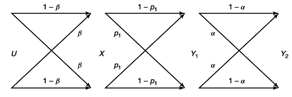
p2 = (1 − p1)α + p1(1 − α) = αp1
βp2 = (1 − p2)β + (1 − β)p2
R1 < I(U;Y2) = H(Y2) − H(Y2|U) = 1 − H(βp2)
R2 < I(X;Y1|U) = H(Y1|U) − H(Y1|X, U) = H(βp1) − H(Y1|X) = H(βp1) − H(p1)
——————————————————————————–——————————————————-
Ben-Guron Univeristy hw2sol.pdf Solution
From the expression for the capacity region, it is clear that the only on trivial possibility for the auxiliary random variable U is that it be binary. From the symmetry of the problem we see that the auxiliary random variable should be connected to X by a binary symmetric channel with parameter β.
Hence we have the setup as shown in figure below:
We can now evaluate the capacity region for this choice of auxiliary random variable. By symmetry best distribution for U is uniform.
\mathchoiceR2R2R2R2 = I(U;Y2) = H(Y2) − H(Y2|U) = H⎛⎝(α)/(2), α, (α)/(2)⎞⎠ − H(Y2|U) = H⎛⎝(α)/(2), α, (α)/(2)⎞⎠ − H((βp + βp)α, α, (βp + β⋅p)⋅α) = (□)
H(Y2|U) = P(U = 0)H(Y2|U = 0) + p(U = 1)H(Y2|U = 1) = H((βp + βp)α, α, (βp + β⋅p)⋅α)
H(Y2|U = 0) = H((βp + βp)α, α, (βp + β⋅p)⋅α) = H(Y2|U = 1) P(U = 0) = P(U = 1) = (1)/(2)
(1 − β)(1 − p)(1 − α) + βp(1 − α) = βpα + βpα = (βp + βp)α
(1 − β)⋅(1 − p)⋅α + (1 − β)⋅p⋅α + β⋅p⋅α + β⋅(1 − p)⋅α = α
(1 − β)⋅p⋅(1 − α) + β(1 − p)(1 − α) = βp⋅α + β⋅p⋅α = (βp + β⋅p)⋅α
(□) = (α)/(2)log(2)/(α) + αlog(1)/(α) + (α)/(2)log(2)/(α) − (β⋅p + β⋅p)⋅α⋅log⎛⎝(1)/((β⋅p + β⋅p)⋅α)⎞⎠ − αlog(1)/(α) − (βp + β⋅p)⋅α⋅log⎛⎝(1)/((βp + β⋅p)⋅α)⎞⎠
(1 − α)log(2)/(1 − α) + αlog(1)/(α) − αlog(1)/(α) − (β⋅p + β⋅p)⋅α⋅log⎛⎝(1)/((β⋅p + β⋅p)⋅α)⎞⎠ − (βp + β⋅p)⋅α⋅log⎛⎝(1)/((βp + β⋅p)⋅α)⎞⎠
\oversetH(α)(1 − α)log(1)/(1 − α) + αlog(1)/(α) − αlog(1)/(α) + (1 − α)log2 + (β⋅p + β⋅p)⋅α⋅log⎛⎝(1)/((β⋅p + β⋅p)⋅α)⎞⎠ + (βp + β⋅p)⋅α⋅log⎛⎝(1)/((βp + β⋅p)⋅α)⎞⎠
H(α) − αlog(1)/(α) + \oversetα(1 − α) − (β⋅p + β⋅p)⋅α⋅log⎛⎝(1)/((β⋅p + β⋅p)⋅α)⎞⎠ − (βp + β⋅p)⋅α⋅log⎛⎝(1)/((βp + β⋅p)⋅α)⎞⎠ = (△)
1 − (β⋅p + β⋅p) = 1 − (1 − β)(1 − p) − βp = 1 − (1 − p − β + βp) − βp = 1 − 1 + p + β − βp − βp = p + β − 2βp
(βp + β⋅p) = (1 − β)p + β(1 − p) = p − βp + β − βp = p + β − 2βp
Значи:
\mathchoice(βp + β⋅p) = 1 − (β⋅p + β⋅p)(βp + β⋅p) = 1 − (β⋅p + β⋅p)(βp + β⋅p) = 1 − (β⋅p + β⋅p)(βp + β⋅p) = 1 − (β⋅p + β⋅p)
(△) = H(α) − αlog(1)/(α) + αH⎛⎝(1)/(2)⎞⎠ − \underset − αH((βp + β⋅p))(β⋅p + β⋅p)⋅α⋅log⎛⎝(1)/((β⋅p + β⋅p))⎞⎠ − (βp + β⋅p)⋅α⋅log⎛⎝(1)/((βp + β⋅p))⎞⎠ − (β⋅p + β⋅p)⋅α⋅log(1)/(α) − (βp + β⋅p)⋅α⋅log(1)/(α) =
H(α) − αlog(1)/(α) + αH⎛⎝(1)/(2)⎞⎠ − \undersetαH((βp + β⋅p)) − (β⋅p + β⋅p)⋅α⋅log(1)/(α) − (βp + β⋅p)⋅α⋅log(1)/(α) =
H(α) − αlog(1)/(α) + αH⎛⎝(1)/(2)⎞⎠ − \undersetαH((βp + β⋅p)) − (1 − \cancel(βp + β⋅p))⋅α⋅log(1)/(α) − \cancel(βp + β⋅p)⋅α⋅log(1)/(α) =
H(α) + αlog(1)/(α) + αH⎛⎝(1)/(2)⎞⎠ − \undersetαH((βp + β⋅p)) − α⋅log(1)/(α) = H(α) − H(α) + + αH⎛⎝(1)/(2)⎞⎠ − \undersetαH((βp + β⋅p)) = \mathchoiceα⋅(1 − H((βp + β⋅p)))α⋅(1 − H((βp + β⋅p)))α⋅(1 − H((βp + β⋅p)))α⋅(1 − H((βp + β⋅p)))
\mathchoiceR1R1R1R1 = I(X;Y1|U) = H(Y1|U) − H(Y1|U, X) = H(Y1|U) − H(Y1|X) = \mathchoice\overset(*)H(βp + βp) − H(p)\overset(*)H(βp + βp) − H(p)\overset(*)H(βp + βp) − H(p)\overset(*)H(βp + βp) − H(p)
Еквивалентата crossover probability за првите два сегменти од каскадата е:
(*) (1 − β)p + β(1 − p) = βp + βp
These equations characterize the boundary of the capacity region as β varies. When β = 0, then R1 = 0 and R2 = α(1 − H(p)). When β = (1)/(2), we have R1 = 1 − H(p) and R2 = 0.
(1)/(2)(1 − p) + (1)/(2)p = (1)/(2) → H(βp + βp) = H⎛⎝(1)/(2)⎞⎠ = 1
βp + βp = (1)/(2)p + (1)/(2)(1 − p) = (1)/(2)
1.12.14 Channels with unknown parameters
We are given a binary symmetric channel with parameter p. The capacity is C = 1 − H(p). Now we change the problem slightly. The receiver knows only that p ∈ {p1, p2} (i.e., p = p1 or p = p2, where p1 and p2 are given real numbers). The transmitter knows the actual value of p. Devise two codes for use by the transmitter, one to be used if p = p1, the other to be used if p = p2, such that transmission to the receiver can take place at rate ≈ C(p1) if p = p1 and at rate ≈ C(p2) if p = p2. (Hint: Devise a method for revealing p to the receiver without affecting the asymptotic rate. Prefixing the codeword by a sequence of 1’s of appropriate length should work.)
EIT Solution Complete
We have two possibilities; the channel is a BSC with parameter p1 or a BSC with parameter p2. If both sender and receiver know that state of channel, then we can achieve the capacity corresponding to which channel is in use, i.e., 1 − H(p1) or 1 − H(p2).
If the receiver does not know the state of the channel, then he cannot know which codebook is being used by the transmitter. He cannot then decode optimally; hence he cannot achieve the rates corresponding to the capacities of the channel.
But the transmitter can inform the receiver of the state of the channel so that the receiver can decode optimally. To do this, the transmitter can precede the codewords by a sequence of 1’s and 0’s. Let us say we use a string of m 1’s to indicate that the channel was in state p1 and m 0’s to indicate state p2. Then, if m = o(n) and m → ∞, where n is the block length of the code used, we have the probability of error in decoding the state of the channel going to zero. Since the receiver will then use the right code for the rest of the message, it will be decoded correctly with P(n)e → 0.
The effective rate for this code is:
R = (log2nC(pi))/(n + m) → C(pi) since m = o(n)
So we can achieve the same asymptotic rate as if both sender and receiver knew the state of the channel.
1.12.15 Two way channel
Consider the tow-way channel shown in bellow. The outputs Y1 and Y2 depend only on the current inputs X1 and X2.\begin_inset Separator latexpar\end_inset
Обратно се стрелките за X2 и Y2 .
(a) By using independently generated codes for the two senders, show that the following rate regions is achievable:
for some product distribution p(x1)p(x2)p(y1y2|x1x2).
(b) Show that the rates for any code for a two-way channel with arbitrarily small probability of error must satisfy (converse).
for some joint distribution p(x1x2)p(y1, y2|x1x2).
The inner and outer bounds on the capacity of the two-way channel are due to Shannon
[3]. He also showed that the inner bound and the outer bound do not coincide in the case of the binary multiplying channel
X1 = X2 = Y1 = Y2 = {0, 1}, Y1 = Y2 = X1, X2 . The capacity of the two-way channel is still and open problem.
(a)
——————————————————————————–——————————————————————————–—————–
nR1 = H(W1) = I(W1;Yn2) + H(W1|Yn2) ≤ I(W1;Yn2) + nϵn ≤ I(Xn1;Yn2) + nϵn ≤ H(Yn2) − H(Yn2|Xn1Xn2) = n⎲⎳i = 1H(Y2i|Yi − 12) − n⎲⎳i = 1H(Y2i|Yi − 12Xn1)
= ∑ni = 1H(Y2i|Yi − 12) − ∑ni = 1H(Y2i|X1iX2i) ≤ ∑ni = 1H(Y2i) − ∑ni = 1H(Y2i|X1iX2i) = ∑ni = 1H(Y2i|X2i) − ∑ni = 1H(Y2i|X1iX2i) = ∑ni = 1I(X1i;Y2i|X2i)
——————————————————————————–——————————————————————————–—————————————————–
nR1 = H(W1) = I(W1;Yn2) + H(W1|Yn2) ≤ I(W1;Yn2) + nϵn ≤ I(Xn1(W1);Yn2) + nϵn = H(Xn1) − H(Xn1|Yn2Xn2)\overset(a) ≤ H(Xn1) − H(Xn1|Yn2Xn2) = H(Xn1|Xn2) − H(Xn1|Yn2Xn2) ≤
≤ ∑ni = 1H(X1i|Xi − 11Xn2) − ∑ni = 1H(X1i|Yn2X1 − i1Xn2) = ∑ni = 1H(X1i|X2i) − ∑ni = 1H(X1i|X2iY2i) = ∑ni = 1I(X1i;Y2i|X2i)
(a) Conditioning reduces entropy
(b) X1 and X2 are independent.
——————————————————————————–——————————————————————————–——————————————————-
Achievability
Recall for Multiple-access channel (Самостојно изведување)
Eij = P(X1i, X2j, Y2 ∈ A(n)ϵ)
Pe = P(Ec11) + ⎲⎳j ≠ 1P(E1i) + ⎲⎳i ≠ 1P(Ei1) + ⎲⎳i ≠ 1P(Ei1) + ⎲⎳i ≠ 1, j ≠ 1P(Eij) = ϵ + ⎲⎳j ≠ 1P(E1i) + ⎲⎳i ≠ 1P(Ei1) + ⎲⎳j ≠ 1P(E1j) + ⎲⎳i ≠ 1, j ≠ 1P(Eij)
P(Ei1) = ⎲⎳x1x2y ∈ A(n)ϵp(x1, x2, y) = ⎲⎳x1x2y ∈ A(n)ϵp(x1)p(x2y) ≤ ⎲⎳x1x2y ∈ A(n)ϵ2 − n(H(X1) − ϵ)2 − n(H(X2Y) − ϵ) ≤ 2n(H(X1X2, Y) + ϵ)2 − n(H(X1) − ϵ)2 − n(H(X2Y) − 2ϵ) =
2n(H(X1X2, Y) + 3ϵ − H(X1) − H(X2Y)) = 2 − n( − H(X1X2Y) − 3ϵ + H(X1) + H(X2Y)) = 2 − n(I(X1;Y|X2) − 3ϵ)
p(x1, x2, y) = p(x1)p(x2|x1)p(y|x1x2) = p(x1)p(x2)p(y|x1x2) = p(x1)p(x2)p(y|x1x2) = p(x1)p(x2y)
− H(X1, X2, Y) + H(X1) + H(X2Y) = − \cancelH(X1) − H(X2|X1) − H(Y|X1X2) + \cancelH(X1) + H(X2) + H(Y|X2) = − \cancelH(X2) − H(Y|X1X2) + \cancelH(X2) + H(Y|X2)
− H(Y|X1X2) + H(Y|X2) = I(X1;Y|X2)
∑j ≠ 1P(E1j) ≤ 2nR1⋅2 − n(I(X1;Y|X2) − 3ϵ)
R1 ≤ I(X1;Y|X2) → if n → ∞ → P(Ei1) → 0
Слично важи за членот
∑ј ≠ 1P(E1 ј) ≤ 2nR2⋅2 − n(I(X2;Y|X1) − 3ϵ) → R2 ≤ I(X2;Y|X1)
односно за членот
∑i ≠ 1, j ≠ 1P(Eij) ≤ 2n(R1 + R2)⋅2 − n(I(X1, X2;Y) − 3ϵ) → R1 + R2 ≤ I(X1, X2;Y)
——————————————————————————–———————————————————-
Eij = P(X1i, X2j, Y1i, Y2j ∈ A(n)ϵ)
Pe = P(Ec11) + ⎲⎳j ≠ 1P(E1i) + ⎲⎳i ≠ 1P(Ei1) + ⎲⎳i ≠ 1P(Ei1) + ⎲⎳i ≠ 1, j ≠ 1P(Eij) = ϵ + ⎲⎳j ≠ 1P(E1i) + ⎲⎳i ≠ 1P(Ei1) + ⎲⎳j ≠ 1P(E1j) + ⎲⎳i ≠ 1, j ≠ 1P(Eij)
P(Ei1) = ⎲⎳(x1x2y1y2) ∈ A(n)ϵp(x1y2|x2)p(x2y1|x1) = ⎲⎳(x1x2y1y2) ∈ A(n)ϵp(x1y2|x2)p(x2y1|x1) ≤ ⎲⎳(x1x2y1y2) ∈ A(n)ϵ2 − n(H(X1Y2|X2) − 2ϵ)2 − n(H(X2Y1|X1) − 2ϵ) ≤
2n(H(X1X2, Y1, Y2) + ϵ)2 − n(H(X1Y2|X2) − ϵ)2 − n(H(X2Y1|X1) − ϵ)
2n(H(X1X2, Y1) + 5ϵ − H(X1Y2|X2) − H(X2Y1|X1)) = 2 − n( − H(X1X2Y1Y2) − 5ϵ + H(X1Y2|X2) + H(X2Y1|X1)) = 2 − n(I(X1;Y2|X2) − 5ϵ)
p(x1, x2, y1, y2) = p(x1)p(x2|x1)p(y1y2|x1x2) = p(x1)p(x2)p(y1|x1x2)p(y2|x1x2y2) = p(x1)p(x2)p(y1|x1x2)p(y2|x1x2) = p(x1y2|x2)p(x2y1|x1)
∑j ≠ 1P(E1j) ≤ 2nR1⋅2 − n(I(X1;Y|X2) − 3ϵ)
R1 ≤ I(X1;Y|X2) → if n → ∞ → P(Ei1) → 0
H(X1X2Y1Y2) + H(X1Y2|X2) + \mathchoiceH(X2Y1|X1)H(X2Y1|X1)H(X2Y1|X1)H(X2Y1|X1) = − H(X1) − H(X2|X1) − H(Y1Y2|X1X2) + H(X1Y2|X2) + H(X2Y1|X1)
H(X1X2Y1Y2) − 5ϵ + H(X1Y2|X2) + H(X2Y1|X1)
H(X1X2Y1Y2) = H(X2) + H(Y1|X2) + H(X1Y2|Y1X2)
H(X1X2Y1Y2) + H(X1Y2|X2) + H(X2Y1|X1) = − H(X2) − H(Y1|X2) − H(X1Y2|Y1X2) + H(X1Y2|X2) + H(X2Y1|X1)
H(X1X2Y1Y2) = H(X1) + H(X2Y1|X1) + H(Y2|X1Y1X2)
H(X1X2Y1Y2) + H(X1Y2|X2) + H(X2Y1|X1) = − H(X1) − \cancelH(X2Y1|X1) − H(Y2|X1Y1X2) + H(X1Y2|X2) + \cancelH(X2Y1|X1) =
= − H(X1) − H(Y2|X1Y1X2) + H(X1Y2|X2) = − \cancelH(X1) − H(Y2|X1Y1X2) + \cancelH(X1|X2) + H(Y2|X1X2) = − H(Y2|X1Y1X2) + H(Y2|X1X2) = I(Y1;Y2|X1X2)
R1 ≤ I(Y1;Y2|X1X2)
——————————————————————————–———————————————————
We will only outline the proof of achievability. It is quite straightforward compared to the more complex channels considered in the text.
Fix p(x1)p(x2)p(y1y2|x1x2)
Code generation:
Generate a cod of size 2nR1 of codewords X1(w1), where the x1i are generated i.i.d. ~ p(x1) . Similarly generate a codebook X2(w2) of size 2nR2 .
To send index w1 form sender 1, he sends X1(w1) . Similarly sender 2 sends X2(w2).
Receiver 1 looks for the unique w2, such that (X1(w1), X2(w2), Y1) ∈ A(n)ϵ(X1X2Y1). If there is no such w2 or more than one such, it declares an error. Similarly, receiver 2 looks for the unique w1, such that (X1(w1), X2(w2), Y2) ∈ A(n)ϵ(X1X2Y2).
Analysis of probability of error
We will only analyze the probability of error in receiver 1. The analysis in receiver 2 is similar.
Without loss of generality, by the symmetry of the random code construction, we can assume that (1, 1) was sent. We have and error at receiver 1if
- (X1(1), X2(1), Y1) ≠ A(n)ϵ(X1X2Y1) The probability of this goes to 0 by the law of large numbers as n → ∞.
- There exist and j ≠ 1 , such that (X1(1), X2(j), Y1) ∈ A(n)ϵ(X1X2Y1)
Define events
Ej = {(X1(1), X2(j), Y1) ∈ A(n)ϵ}
Then by the union of events bound,
P(n)ϵ = P(Ec1∪∪j ≠ 1Ej) ≤ P(Ec1) + ∑j ≠ 1P(Ej)
where P is the probability given that (1, 1) was sent. From AEP, P(Ec1) → 0.
P(Ej) = P((X1X2(j), Y1) ∈ A(n)ϵ) = ∑x1x2yp(x2)p(x1y1) ≤ |A(n)ϵ|2 − n(H(X2) − ϵ)2 − n(H(X1Y1) − ϵ) ≤ 2n(H(X1X2Y1) − ϵ)2 − n(H(X2) − ϵ)2 − n(H(X1Y1) − ϵ)
= 2 − n(I(X2;X1Y) − 3ϵ) = 2 − n(I(X2;Y|X1) − 3ϵ)
I(X2;X1Y) = \cancelI(X2;X1) + I(X2;Y|X1) = I(X2;Y|X1)
since X1X2 are independent.
Therefore
P(n)e ≤ ϵ + 2nR22 − n(I(X2;Y|X1) − 3ϵ)
R2 ≤ I(X2;Y|X1) → n → ∞ → Pe → 0
(b) The converse is a simple application of the general Tehorem 15.10.1 to this simple case. The sets S can be taken in turn ot be ech node. We will not go into the details.
1.12.16 Multiple-access channel
Let the output Y of a multiple access channel be given by
where X1, X2 are both real and power limited,
and
sgn(x) = ⎧⎨⎩
1
x > 0
− 1
x ≤ 0
Note that there is interference but no noise in this channel.
(a) Find the capacity region.
(b) Describe a coding scheme that achieves the capacity region.
——————————————————————————–———————–
R1 < I(X1;Y|X2) R2 < I(X2;Y|X1) R1 + R2 < I(X1X2;Y)
I(X1;Y|X2) = ?
——————————————————————————–——–
recall for gaussian channel
Y = X1 + X2 + Z
I(X1;Y|X2) = H(Y|X2) − H(Y|X1X2) = H(X1 + X2 + Z|X2) − H(X1 + X2 + Z|X1X2) ≤ (1)/(2)log22πe(P1 + N) − (1)/(2)log22πe(N) =
= (1)/(2)log2⎛⎝1 + (P1)/(N)⎞⎠ = C⎛⎝(P1)/(N)⎞⎠ → R1 < C⎛⎝(P1)/(N)⎞⎠
R2 < C⎛⎝(P2)/(N)⎞⎠
I(X1X2;Y) = H(Y) − H(Y|X1X2) = H(X1 + X2 + Z) − H(X1 + X2 + Z|X1X2) ≤ (1)/(2)log22πe(P1 + P2 + N) − (1)/(2)log22πe(N) =
= (1)/(2)log2⎛⎝1 + (P1 + P2)/(N)⎞⎠ = C⎛⎝(P1 + P2)/(N)⎞⎠ → R1 + R2 < C⎛⎝(P1 + P2)/(N)⎞⎠
——————————————————————————–———–
Y = X1 + sgn(X2)
I(X1;Y|X2) = H(Y|X2) − H(Y|X1X2) = H(X1 + sgn(X2)|X2) − H(X1 + sgn(X2)|X1X2) = H(X1) ≤ (1)/(2)log22πe(P1)
R1 < (1)/(2)log22πe(P1)
I(X2;Y|X1) = H(Y|X1) − H(Y|X1X2) = H(X1 + sgn(X2)|X1) − H(X1 + sgn(X2)|X1X2) = H(sgn(X2))
≤ (1)/(2)log22πe(E(sgn(X2)2)) = (1)/(2)log2(2πe)
R2 < (1)/(2)log22πe
I(X1X2;Y) = H(Y) − H(Y|X1X2) = H(X1 + sgn(X2)) − H(X1 + sgn(X2)|X1X2) ≤ (1)/(2)log22πe(P1 + 1) = (1)/(2)log2(P1 + 1)
R1 + R2 < (1)/(2)log2(P1 + 1)
——————————————————————————–———————–
EIT Solutions Complete
(a) This is continuous noiseless multiple access channel, if we let U2 = sgn(X2) we can consider a channel form X1 and U2 to Y.
I(X1;Y|X2) = h(Y|X2) − h(Y|X1X2) = h(X1 + U2|X2) − h(X1 + U2|X1X2) = h(X1) − ( − ∞) = ∞
since X1 and X2 are independent and similarly
I(X2;Y|X1) = I(X2, U2;Y|X1) = I(U2;Y|X1) + I(X2;Y|X1, U2) = I(U2;Y|X1) = H(U2) − H(U2|Y, X1) ≤ H⎛⎝(1)/(2)⎞⎠ = 1
Ова ме потсеќа на distortion rate, т.е. sgn(X2) е репрезентација на X2 .
I(X, f(X);Y) = H(Y) − H(Y|X, f(X)) = H(Y) − H(Y|X) = I(X, Y)
I(X2;Y|X1, U2) = H(Y|X1U2) − H(Y|X1U2X2) = H(Y|X1U2) − H(Y|X1X2) = 0
I(X1, X2;Y) = h(Y) − h(Y|X1X2) = h(Y) − ( − ∞) = ∞
Thus we can send at infinite rate form X1 to Y and at a maximum rate of 1 bit/transmission from X2 to Y
(b) We can senda a 1 for X2 in fist transmission, and knowing this, Y can recover X1 perfectly, recovering an infinite number of bits. From then on, X1 can be 0 and we can send 1 bit per transmission using the sign of X2.
Let (X, Y) have joint probability mass function p(x, y)
p(x, y)
1
2
3
1
α
β
β
2
β
α
β
3
β
β
α
where β = (1)/(6) − (α)/(2). (Note: This is joint, not conditional, probability mass function.)
(a) Find the Slepian-Wolf rate region for this source.
(b) What isPr{X = Y} in terms of α?
(c) What is the rate region if α = (1)/(3)?
(d) What is the rate region if α = (1)/(9)?
——————————————————————————–——————————————————–
R1 ≥ H(X|Y) R2 ≥ H(Y|X) R1 + R2 ≥ H(X, Y)
p(x, y)
1
2
3
p(x)
1
α
β
β
α + 2β
2
β
α
β
α + 2β
3
β
β
α
α + 2β
p(y)
α + 2β
α + 2β
α + 2β
p(x|y)
1
2
3
1
(α)/(α + 2β)
(β)/(α + 2β)
(β)/(α + 2β)
2
(β)/(α + 2β)
(α)/(α + 2β)
(β)/(α + 2β)
3
(β)/(α + 2β)
(β)/(α + 2β)
(α)/(α + 2β)
(a)
H(X|Y) = H(Y|X) = 3αlog2⎛⎝(α + 2β)/(α)⎞⎠ + 6β⋅log2⎛⎝(α + 2β)/(β)⎞⎠
H(X|Y) = (1)/(2)⋅⎛⎝(3 − 9 α)log2⎛⎝(2)/((1 − 3⋅α))⎞⎠ + 6 α log2⎛⎝(1)/(3⋅α)⎞⎠⎞⎠
H(X, Y) = 3αlog2⎛⎝(1)/(α)⎞⎠ + 6β⋅log2⎛⎝(1)/(β)⎞⎠ = 3αlog2⎛⎝(1)/(α)⎞⎠ + 6⎛⎝(1 − 3α)/(6)⎞⎠⋅log2⎛⎝(6)/(1 − 3⋅α)⎞⎠
(b)
Pr{X = Y} = p(X = 1)⋅p(Y = 1|X = 1) + p(X = 2)⋅p(Y = 2|X = 2) + p(X = 3)⋅p(Y = 3|X = 3)
= ∑3i = 1p(X = i)p(Y = i|X = i) = 3\cancel(α + 2β)⋅(α)/(\cancel(α + 2β)) = 3⋅α
(c)
H(X|Y) = H(Y|X) = 0
H(X, Y) = log2(3)
R1 ≥ 0 R2 ≥ 0 R1 + R2 ≥ log2(3)
(d)
H(X|Y) = H(Y|X) = log2(3)
H(X, Y) = H(X, Y) = 2log2(3)
R1 ≥ log2(3) R2 ≥ log2(3) R1 + R2 ≥ 2⋅log2(3)
——————————————————————————–——————————————————————————–——————————————————————-
EIT Complete solutions
H(X, Y) = 3αlog2⎛⎝(1)/(α)⎞⎠ + 6β⋅log2⎛⎝(1)/(β)⎞⎠ = 3αlog2⎛⎝(1)/(3α)⎞⎠ + 3β⋅log2⎛⎝(1)/(3β)⎞⎠ + 3β⋅log2⎛⎝(1)/(3β)⎞⎠ + 3αlog(3) + 6βlog(3)
= 3αlog2⎛⎝(1)/(3α)⎞⎠ + 3β⋅log2⎛⎝(1)/(3β)⎞⎠ + 3β⋅log2⎛⎝(1)/(3β)⎞⎠ + \underset1(3α + 6β)⋅log(3) = H(3α, 3β, 3β) + log(3)
H(X|Y) = H(Y|X) = 3αlog2⎛⎝(α + 2β)/(α)⎞⎠ + 6β⋅log2⎛⎝(α + 2β)/(β)⎞⎠ = 3αlog2⎛⎝(1)/(3α)⎞⎠ + 6β⋅log2⎛⎝(1)/(3β)⎞⎠ = 3αlog2⎛⎝(1)/(3α)⎞⎠ + 3β⋅log2⎛⎝(1)/(3β)⎞⎠ + 3β⋅log2⎛⎝(1)/(3β)⎞⎠ = H(3α, 3β, 3β)
Исти резултати се добиваат само што овие се прикажани во покомпактна форма . Исто така јас не забележав дека важат
158↑ и
159↑.
——————————————————————————–——————————————————————————–———————————————————————
1.12.18 Square channel
What is the capacity of the following multiple access channels
X1 ∈ { − 1, 0, 1} X2 ∈ { − 1, 0, 1} Y = X21 + X22
(a) Find the capacity region
(b) Describe p*(x1), p*(x2) achieving a point on the boundary of the capacity region
(a)
Y ∈ {0, 1, 2}
I(X1, X2, Y) = H(Y) − H(Y|X1X2) = H(X21 + X22) ≤ log(3) = 1.585
X2 ∈ {0, 1}
R1 < I(X1;Y|X2) = H(Y|X2) − H(Y|X2X1) = H(X21 + X22|X2) − H(X21 + X22|X1X2) = H(X21 + X22|X2) = H(X21) ≤ log2(2) = 1
R2 < I(X2;Y|X1) = H(Y|X1) − H(Y|X2X1) = H(X21 + X22|X1) − H(X21 + X22|X1X2) = H(X21 + X22|X1) = H(X22) ≤ log2(2)
(b)
p(X21) ~ ⎧⎩(1)/(2), (1)/(2)⎫⎭ p(X1) = ?
X21 ∈ {0, 1} X1 ∈ { − 1, 0, 1} p(X1) = ⎧⎩(1)/(4), (1)/(2), (1)/(4)⎫⎭
X22 ∈ {0, 1} X2 ∈ { − 1, 0, 1} p(X2) = ⎧⎩(1)/(4), (1)/(2), (1)/(4)⎫⎭
(a)
If we let U1 = X21 and U2 = X22 , then he channel is equivalent to a sum multiple access channel Y = U1 + U2 . We could aso get the same beahviour by using only two input symbols (0 and 1) for both X1 and X2.
Thus the capacity region is
R1 < I(X1;Y|X2) = H(Y|X2)
R2 < I(X2;Y|X1) = H(Y|X1)
R1 + R2 < I(X1X2;Y) = H(Y)
Со избирање на
p(x1x2) = (1)/(4) for
(x1x2) = (1, 0), (0, 0), (0, 1), (1, 1) and
0 otherwise, we obtain
p(x1x2) p(x2|x1)
x1|x2
− 1
0
1
p(x2)
− 1
0
0
0
0
0
0.25
0.25
0.5
1
0
0.25
0.25
0.5
p(X1)
0
0.5
0.5
x1|x2
− 1
0
1
p(x2)
− 1
0
0
0
0
0
0.125
0.125
0.5
1
0
0.125
0.125
0.5
p(X1)
0
0.5
0.5
H(Y|X1) = p(X1 = 0)H(Y|X1 = 0) + p(X1 = 1)H(Y|X1 = 1) = (1)/(2)⋅1 + (1)/(2)⋅1 = 1
H(Y|X1 = 0) = p(Y = 0|X1 = 0)⋅log⎛⎝(1)/(p(Y = 0|X1 = 0))⎞⎠ + p(Y = 1|X1 = 0)⋅log⎛⎝(1)/(p(Y = 1|X1 = 0))⎞⎠ + \overset0p(Y = 2|X1 = 0)⋅log⎛⎝(1)/(p(Y = 2|X1 = 0))⎞⎠
H(Y|X1 = 0) = 2⋅(1)/(4)⋅log4 = 1
H(Y|X1 = 1) = \overset0p(Y = 0|X1 = 1)⋅log⎛⎝(1)/(p(Y = 0|X1 = 1))⎞⎠ + p(Y = 1|X1 = 1)⋅log⎛⎝(1)/(p(Y = 1|X1 = 1))⎞⎠ + p(Y = 2|X1 = 01)⋅log⎛⎝(1)/(p(Y = 2|X1 = 0))⎞⎠
H(Y|X1 = 1) = 2⋅(1)/(4)⋅log4 = 1
p(Y = 0|X1 = 0) = p(X2 = 0, X1 = 0) = (1)/(4)
p(Y = 1|X1 = 0) = p(X2 = 1, X1 = 0) = (1)/(4)
p(Y = 2|X1 = 0) = 0
p(Y = 0|X1 = 1) = p(X2 = 0, X1 = 1) = 0
p(Y = 1|X1 = 1) = p(X2 = 0, X1 = 1) = (1)/(4)
p(Y = 2|X1 = 1) = p(X2 = 1, X1 = 1) = (1)/(4)
Подобар пристап (наместо овој во box-от) за пресметка на неизвесноста на Y кога за дадено X e:
(Глеадај ја табелата за здружена веојатност)
H(Y|X1 = 0) = H(X1 + X2|X1 = 0) = H(X2|X1 = 0) = (1)/(4)⋅2 + (1)/(4)⋅2 = 1
H(Y|X1 = 1) = H(X1 + X2|X1 = 1) = H(X2|X1 = 1) = (1)/(4)⋅2 + (1)/(4)⋅2 = 1
Y ∈ {0, 1, 2}
H(Y) = H(p(Y = 0), p(Y = 1), p(Y = 2))
p(Y = 1) = p(X1 = 0, X2 = 1) + p(X1 = 1, X2 = 0) = 0.5
p(Y = 0) = p(X1 = 0, X2 = 0) = 0.25
p(Y = 2) = p(X1 = 1, X2 = 1) = 0.25
H(Y) = 2⋅(1)/(4)log(4) + (1)/(2)⋅log2 = 1 + 0.5 = 1.5
(b)
The possible distribution that achieves points on the boundary of the rate region is given by the distribution in part (a)
Two senders know random variables U1 and U2, respectively. Let the random variables (U1, U2) have the following joint distribution
U1\U2
0
1
2
...
m − 1
0
α
(β)/(m − 1)
(β)/(m − 1)
...
(β)/(m − 1)
1
(β)/(m − 1)
0
0
0
0
2
(β)/(m − 1)
0
0
0
0
...
...
0
0
0
0
3
(β)/(m − 1)
0
0
0
0
where α + β + γ = 1. Find the region of rates (R1, R2) that would allow common receier to decode both random variables reliably.
——————————————————–
R1 ≥ H(U1|U2) R2 ≥ H(U2|U1) R1 + R2 ≥ H(U1U2)
U1\U2
0
1
2
...
m − 1
p(U2)
0
α
(β)/(m − 1)
(β)/(m − 1)
...
(β)/(m − 1)
α + β
1
(γ)/(m − 1)
0
0
0
0
(γ)/(m − 1)
2
(γ)/(m − 1)
0
0
0
0
(γ)/(m − 1)
...
...
0
0
0
0
m − 1
(γ)/(m − 1)
0
0
0
0
(γ)/(m − 1)
p(U1)
α + γ
(β)/(m − 1)
(β)/(m − 1)
...
(β)/(m − 1)
U1\U2
0
1
2
...
m − 1
p(U2)
0
(α)/(α + β)
(β)/((m − 1)(α + β))
(β)/((m − 1)(α + β))
...
(β)/((m − 1)(α + β))
α + β
1
1
0
0
0
0
(γ)/(m − 1)
2
1
0
0
0
0
(γ)/(m − 1)
...
...
0
0
0
0
m − 1
1
0
0
0
0
(γ)/(m − 1)
p(U1)
α + β
(β)/(m − 1)
(β)/(m − 1)
...
(β)/(m − 1)
p(U1) = α + β + (m − 1)(β)/(m − 1) = α + 2β = 1
p(U2) = α + β + (m − 1)(γ)/(m − 1) = α + β + γ = 1
\mathchoiceH(U1U2)H(U1U2)H(U1U2)H(U1U2) = αlog⎛⎝(1)/(α)⎞⎠ + (m − 1)(γ)/(m − 1)⋅log((m − 1))/(γ) + (m − 1)(β)/(m − 1)⋅log((m − 1))/(β) = αlog⎛⎝(1)/(α)⎞⎠ + γ⋅log((m − 1))/(γ) + β⋅log((m − 1))/(β)
= αlog⎛⎝(1)/(α)⎞⎠ + γ⋅log((m − 1))/(γ) + β⋅log((m − 1))/(β) = \mathchoiceH(α, β, γ) + (γ + β)log(m − 1)H(α, β, γ) + (γ + β)log(m − 1)H(α, β, γ) + (γ + β)log(m − 1)H(α, β, γ) + (γ + β)log(m − 1)
\mathchoiceH(U1|U2)H(U1|U2)H(U1|U2)H(U1|U2) = H(U1U2) − H(U2) = H(α, β, γ) + (γ + β)log(m − 1) − (α + β)⋅log⎛⎝(1)/(α + β)⎞⎠ − (m − 1)(γ)/(m − 1)⋅log((m − 1))/(γ)
H(α, β, γ) + (γ + β)log(m − 1) − (α + β)⋅log⎛⎝(1)/(α + β)⎞⎠ − γ⋅log((m − 1))/(γ) = H(α, β) + (γ + β)log(m − 1) − (α + β)⋅log⎛⎝(1)/(α + β)⎞⎠ − γ⋅log(m − 1)
\mathchoiceH(α, β) + βlog(m − 1) − (α + β)⋅log⎛⎝(1)/(α + β)⎞⎠H(α, β) + βlog(m − 1) − (α + β)⋅log⎛⎝(1)/(α + β)⎞⎠H(α, β) + βlog(m − 1) − (α + β)⋅log⎛⎝(1)/(α + β)⎞⎠H(α, β) + βlog(m − 1) − (α + β)⋅log⎛⎝(1)/(α + β)⎞⎠
\mathchoiceH(U2|U1)H(U2|U1)H(U2|U1)H(U2|U1) = H(U1U2) − H(U1) = H(α, β, γ) + (γ + β)log(m − 1) − (α + γ)⋅log⎛⎝(1)/(α + γ)⎞⎠ − (m − 1)(β)/(m − 1)⋅log((m − 1))/(β)
H(α, β, γ) + (γ + β)log(m − 1) − (α + γ)⋅log⎛⎝(1)/(α + γ)⎞⎠ − β⋅log((m − 1))/(β) = H(α, γ) + (γ + β)log(m − 1) − (α + γ)⋅log⎛⎝(1)/(α + γ)⎞⎠ − β⋅log(m − 1)
\mathchoiceH(α, γ) + γlog(m − 1) − (α + γ)⋅log⎛⎝(1)/(α + γ)⎞⎠H(α, γ) + γlog(m − 1) − (α + γ)⋅log⎛⎝(1)/(α + γ)⎞⎠H(α, γ) + γlog(m − 1) − (α + γ)⋅log⎛⎝(1)/(α + γ)⎞⎠H(α, γ) + γlog(m − 1) − (α + γ)⋅log⎛⎝(1)/(α + γ)⎞⎠
1.12.20 Multiple access
(a) Find the capacity region for the multiple access channel
where
X1 ∈ {2, 4}, X2 ∈ {1, 2}
(b) Suppose that the range of X1 is {1, 2}. Is the capacity region decreased? Why or why not?
——————————————————————————–——————————————————————————-
p(Y|X1X2) p(X1X2Y)
X1X2|Y
2
4
16
(2, 1)
1
0
0
(2, 2)
0
1
0
(4, 1)
0
1
0
(4, 2)
0
0
1
X1X2|Y
2
4
16
p(X1X2)
(2, 1)
1 ⁄ 3
0
0
1 ⁄ 3
(2, 2)
0
1 ⁄ 6
0
1 ⁄ 6
(4, 1)
0
1 ⁄ 6
0
1 ⁄ 6
(4, 2)
0
0
1 ⁄ 3
1 ⁄ 3
p(Y)
1 ⁄ 3
1 ⁄ 3
1 ⁄ 3
R1 + R2 ≤ I(X1, X2;Y) = H(Y) − H(Y|X1X2) = H(Y) = log3 = 1.585
R1 ≤ I(X1;Y|X2) = H(Y|X2) − H(Y|X1X2) = H(Y|X2) = (1)/(2)log3 + (1)/(6) = 1.432
R1 ≤ I(X2;Y|X1) = H(Y|X1) − H(Y|X1X2) = H(Y|X1) = (1)/(2)log3 + (1)/(6) = 1.432
log[3.0] + (1)/(3) = 1.43195
p(Y = 2) = p(X1 = 2, X2 = 1) p(Y = 16) = p(X1 = 4, X2 = 2) p(Y = 4) = p(X1 = 2, X2 = 2) + p(X1 = 4, X2 = 1)
p(Y = 2) = p(Y = 16) = (1)/(3) p(Y = 4) = (1)/(3) p(X1 = 2, X2 = 2) = p(X1 = 4, X2 = 1) = (1)/(6)
H(Y) = 3⋅(1)/(3)log(3) = log(3) = 1.585
————————————————————
H(Y|X1) = p(X1 = 2)H(Y|X1 = 2) + p(X1 = 4)H(Y|X1 = 4)
H(Y|X1 = 2) = H(2X2|X1 = 2) = H(X2|X1 = 2) = (1)/(3)log(3) + (1)/(6)log(6) = (1)/(3)log3 + (1)/(6)log3 + (1)/(6) = ⎛⎝(2 + 1)/(6)⎞⎠log3 + (1)/(6) = (1)/(2)log3 + (1)/(6) =
U = 2X2 ∈ {2, 4}
H(Y|X1 = 4) = H(4X2|X1 = 4) = H(X2|X1 = 4) = (1)/(3)log(3) + (1)/(6)log(6) = (1)/(3)log3 + (1)/(6)log3 + (1)/(6) = ⎛⎝(2 + 1)/(6)⎞⎠log3 + (1)/(6) = (1)/(2)log3 + (1)/(6)
V = 4X2 ∈ {4, 16}
\mathchoiceH(Y|X1)H(Y|X1)H(Y|X1)H(Y|X1) = p(X1 = 2)H(Y|X1 = 2) + p(X1 = 4)H(Y|X1 = 4) =
= ⎛⎝(1)/(2)log3 + (1)/(6)⎞⎠(p(X1 = 2) + p(X1 = 4)) = (1)/(2)log3 + (1)/(6) = \mathchoiceH(X2|X1)H(X2|X1)H(X2|X1)H(X2|X1)
————————————————————
H(Y|X2) = p(X2 = 1)H(Y|X2 = 1) + p(X2 = 2)H(Y|X2 = 2)
H(Y|X2 = 1) = H(XX21|X2 = 1) = H(X1|X2 = 1) = (1)/(3)log(3) + (1)/(6)log(6) = (1)/(3)log3 + (1)/(6)log3 + (1)/(6) = ⎛⎝(2 + 1)/(6)⎞⎠log3 + (1)/(6) = (1)/(2)log3 + (1)/(6) =
X1 ∈ {2, 4}
H(Y|X2 = 2) = H(XX21|X2 = 2) = H(X21|X2 = 2) = H(X1|X2 = 2) = (1)/(3)log(3) + (1)/(6)log(6) =
= (1)/(3)log3 + (1)/(6)log3 + (1)/(6) = ⎛⎝(2 + 1)/(6)⎞⎠log3 + (1)/(6) = (1)/(2)log3 + (1)/(6)
X21 ∈ {4, 16}
\mathchoiceH(Y|X2)H(Y|X2)H(Y|X2)H(Y|X2) = p(X2 = 2)H(Y|X2 = 2) + p(X2 = 4)H(Y|X2 = 4) =
⎛⎝(1)/(2)log3 + (1)/(6)⎞⎠(p(X2 = 2) + p(X2 = 4)) = (1)/(2)log3 + (1)/(6) = \mathchoiceH(X1|X2)H(X1|X2)H(X1|X2)H(X1|X2)
H(X1) = H(X1X2) − H(X2|X1) = log3 + (1)/(3) − (1)/(2)log3 − (1)/(6) = (1)/(2)log3 + (1)/(6) = H(X2)
H(X1X2) = H(X1) + H(X2)
(b)
p(Y|X1X2) p(X1X2Y)
X1X2|Y
1
2
4
(1, 1)
1
0
0
(1, 2)
1
0
0
(2, 1)
0
1
0
(2, 2)
0
0
1
X1X2|Y
1
2
4
p(X1X2)
(1, 1)
1 ⁄ 6
0
0
1 ⁄ 3
(1, 2)
1 ⁄ 6
0
0
1 ⁄ 6
(2, 1)
0
1 ⁄ 3
0
1 ⁄ 6
(2, 2)
0
0
1 ⁄ 3
1 ⁄ 3
p(Y)
1 ⁄ 3
1 ⁄ 3
1 ⁄ 3
R1 + R2 ≤ I(X1, X2;Y) = H(Y) − H(Y|X1X2) = H(Y) = log3
R1 ≤ I(X1;Y|X2) = H(Y|X2) − H(Y|X1X2) = H(Y|X2) = (1)/(2)log3 + (1)/(6)
\mathchoiceR2 ≤ I(X2;Y|X1) = H(Y|X1) − H(Y|X1X2) = H(Y|X1) = ⎛⎝(1)/(2)log3 + (1)/(6)⎞⎠p(X1 = 2) ≤ ⎛⎝(1)/(2)log3 + (1)/(6)⎞⎠R2 ≤ I(X2;Y|X1) = H(Y|X1) − H(Y|X1X2) = H(Y|X1) = ⎛⎝(1)/(2)log3 + (1)/(6)⎞⎠p(X1 = 2) ≤ ⎛⎝(1)/(2)log3 + (1)/(6)⎞⎠R2 ≤ I(X2;Y|X1) = H(Y|X1) − H(Y|X1X2) = H(Y|X1) = ⎛⎝(1)/(2)log3 + (1)/(6)⎞⎠p(X1 = 2) ≤ ⎛⎝(1)/(2)log3 + (1)/(6)⎞⎠R2 ≤ I(X2;Y|X1) = H(Y|X1) − H(Y|X1X2) = H(Y|X1) = ⎛⎝(1)/(2)log3 + (1)/(6)⎞⎠p(X1 = 2) ≤ ⎛⎝(1)/(2)log3 + (1)/(6)⎞⎠
Да!!! Регионот на капацитети се намалува. R2(b) е помало или еднаков на R2(a).
p(Y = 2) = p(X1 = 2, X2 = 1) p(Y = 4) = p(X1 = 4, X2 = 2) p(Y = 1) = p(X1 = 1, X2 = 1) + p(X1 = 1, X2 = 2)
p(Y = 2) = p(Y = 4) = (1)/(3) p(Y = 1) = (1)/(3) p(X1 = 1, X2 = 1) = p(X1 = 1, X2 = 2) = (1)/(6)
H(Y) = 3⋅(1)/(3)log(3) = log(3) = 1.585
————————————————————
H(Y|X1) = p(X1 = 1)H(Y|X1 = 1) + p(X1 = 2)H(Y|X1 = 2)
H(Y|X1 = 1) = H(2X2|X1 = 1) = H(1|X1 = 1) = 0
Y = 1X2 ∈ {1}
H(Y|X1 = 2) = H(2X2|X1 = 2) = H(X2|X1 = 2) = (1)/(3)log(3) + (1)/(3)log(3) = (2)/(3)log3
Y = 2X2 ∈ {2, 4}
H(Y|X1) = p(X1 = 1)⋅0 + p(X1 = 2)H(Y|X1 = 2) = ⎛⎝(1)/(2)log3 + (1)/(6)⎞⎠p(X1 = 2)
————————————————————
H(Y|X2) = p(X2 = 1)H(Y|X2 = 1) + p(X2 = 2)H(Y|X2 = 2)
H(Y|X2 = 1) = H(XX21|X2 = 1) = H(X1|X2 = 1) = − p(Y = 1|X2 = 1)log(p(Y = 1|X2 = 1)) − p(Y = 2|X2 = 1)log(p(Y = 2|X2 = 1))
= (1)/(6)log(6) + (1)/(3)log(3) = (1)/(6)log3 + (1)/(6) + (1)/(3)log3 = ⎛⎝(2 + 1)/(6)⎞⎠log3 + (1)/(6) = (1)/(2)log3 + (1)/(6)
Условните веројатности со Y одговараат на здружените веројатности на сите три променливи.
X1 ∈ {1, 2}
H(Y|X2 = 2) = H(XX21|X2 = 2) = H(X21|X2 = 2) = H(X1|X2 = 2) =
= − p(Y = 1|X2 = 2)log(p(Y = 1|X2 = 2)) − p(Y = 4|X2 = 2)log(p(Y = 4|X2 = 2)) = (1)/(3)log(3) + (1)/(6)log(6) =
= (1)/(3)log3 + (1)/(6)log3 + (1)/(6) = ⎛⎝(2 + 1)/(6)⎞⎠log3 + (1)/(6) = (1)/(2)log3 + (1)/(6)
X21 ∈ {1, 4}
H(Y|X2) = p(X2 = 1)H(Y|X2 = 1) + p(X2 = 2)H(Y|X2 = 2) = ⎛⎝(1)/(2)log3 + (1)/(6)⎞⎠(p(X2 = 1) + p(X2 = 2)) = (1)/(2)log3 + (1)/(6) = H(X1|X2)
H(X1X2Y) = 2(1)/(3)log3 + 2⋅(1)/(6)⋅log6 = (2)/(3)log3 + (1)/(3)log3 + (1)/(3) = log3 + (1)/(3)
With X1 ∈ {2, 4}, X2 ∈ {1, 2}, the channel Y = XX21 behaves as (не ги гледај вредностите во здружента):
X1X2
Y
(2, 1)
2
(2, 2)
4
(4, 1)
4
(4, 2)
16
We compute
R1 ≤ I(X1;Y|X2) = H(Y|X2) − H(Y|X1X2) = H(XX21|X2) = | \refeq:Eq15.352|H(X1|X2) = 1 bits per transmition
R2 ≤ I(X2;Y|X1) = H(Y|X1) − H(Y|X1X2) = H(XX21|X1) = | \refeq:Eq15.353|H(X2|X1) = H(X2) = 1 bits per transmition
R1 + R2 ≤ I(X1X2;Y) = H(Y) − H(Y|X1X2) = H(Y) = (3)/(2) bits per transmition
Во моите изведувања добив повисока вредност за H(Y) = log3 зошто земав Y да биде униформно распределена. Овде изгледа избрале распределбата да биде [p(2, 1), p(2, 2) + p(4, 1), p(4, 2)] = ⎡⎣(1)/(4), (1)/(2), (1)/(4)⎤⎦.
т.е униформна p(x1x2) распределба.
Where the bound
R1 + R2 is achieved at the corners of
16↑, where eaither sender 1 or 2 sends 1 bit per transmission adn the other user treats the channel as a binary erasure cahnnel wiht capacity
1 − perasure = 1 − (1)/(2) = (1)/(2) bits per use of the channel. Other points on the line are achieved by timesharing.
(b)
With X1 ∈ {1, 2}, X2 ∈ {1, 2} , the channel Y = XX21 behaves like (не ги гледај вредностите во здружената)
X1X2
Y
(1, 1)
1
(1, 2)
1
(2, 1)
2
(2, 2)
4
Note when X1 = 1 X2 has no effect on Y and can not be recovered given X1 and Y. If \mathchoiceX1 ~ Br(α)X1 ~ Br(α)X1 ~ Br(α)X1 ~ Br(α) and \mathchoiceX2 ~ Br(β)X2 ~ Br(β)X2 ~ Br(β)X2 ~ Br(β) then:
\mathchoiceR1R1R1R1 ≤ I(X1;Y|X2) = H(Y|X2) − H(Y|X1X2) = H(Y|X2)
H(Y|X2) = p(X2 = 1)H(Y|X2 = 1) + p(X2 = 2)H(Y|X2 = 2) = (*)
***********************************************
X1 ∈ {1, 2}
H(Y|X2 = 1) = H(XX21|X2 = 1) = H(X1|X2 = 1)
***********************************************
X1 ∈ {1, 2} → X21 ∈ {1, 4} се мапираат еден на еден па нема промена на дистрибуцијата со преод на X21
H(Y|X2 = 2) = H(XX21|X2 = 2) = H(X21|X2 = 2) = H(X1|X2 = 2)
************************************************************
(*) = p(X2 = 1)H(X1|X2 = 1) + p(X2 = 2)H(X1|X2 = 2) = H(X1|X2) = H(X1) = \mathchoiceH(α)H(α)H(α)H(α)
**************************************************************
X1X2
Y
(1, 1)
1
(1, 2)
1
(2, 1)
2
(2, 2)
4
\mathchoiceR2R2R2R2 ≤ I(X2;Y|X1) = H(Y|X1) − H(Y|X1X2) = \mathchoiceH(Y|X1)H(Y|X1)H(Y|X1)H(Y|X1)
p(X1 = 1) = α p(X1 = 2) = 1 − α = α p(X2 = 1) = β p(X2 = 2) = 1 − β = β
p(Y = 2) = p(X1 = 2, X2 = 1) = αβ p(Y = 4) = p(X1 = 2, X2 = 2) = αβ p(Y = 1) = p(X1 = 1, X2 = 1) + p(X1 = 1, X2 = 2) = αβ + αβ
———————————————————–
H(Y|X1) = p(X1 = 1)H(Y|X1 = 1) + p(X1 = 2)H(Y|X1 = 2)
H(Y|X1 = 1) = H(2X2|X1 = 1) = H(1|X1 = 1) = 0
Y = 1X2 ∈ {1}
H(Y|X1 = 2) = H(2X2|X1 = 2) = H(X2|X1 = 2)
Y = 2X2 ∈ {2, 4}се мапираат еден на еден па нема промена на дистрибуцијата со преод на X21
\mathchoiceH(Y|X1)H(Y|X1)H(Y|X1)H(Y|X1) = p(X1 = 1)⋅0 + p(X1 = 2)H(Y|X1 = 2) = H(XX21|X1 = 2)p(X1 = 2) = (1 − α)H(2X2|X1 = 2) = (1 − α)H(X2|X1 = 2) =
-(1-α)(p(X2=1|X1=2)logp(X2=1|X1=2)+p(X2=2|X1=2)logp(X2=2|X1=2)) = |не зависни се| = (1 − α)H(X2) = \mathchoice(1 − α)H(β)(1 − α)H(β)(1 − α)H(β)(1 − α)H(β)
\mathchoiceR1 + R2R1 + R2R1 + R2R1 + R2 ≤ I(X1X2;Y) = H(Y) − H(Y|X1X2) = H(Y) = H(αβ, αβ, αβ + αβ) =
− H(αβ, αβ, αβ + αβ) = (1 − α)βlog(1 − α)β + (1 − α)(1 − β)log(1 − α)(1 − β) + (\cancelαβ + (1 − \cancelβ)α)log(αβ + (1 − β)α)
= (1 − α)βlog(1 − α)β + (1 − α)(1 − β)log(1 − α)(1 − β) + (α)log(α)
= (1 − α)βlog(1 − α) + (1 − α)βlogβ + (1 − α)(1 − β)log(1 − α) + (1 − α)(1 − β)log(1 − β) + αlogα
= (1 − α)βlog(1 − α) + αlogα + (1 − α)βlogβ + (1 − α)(1 − β)log(1 − α) + (1 − α)(1 − β)log(1 − β)
= (1 − α)βlog(1 − α) + αlogα + βlogβ − αβlogβ + (1 − α)(1 − β)log(1 − α) + (1 − α)(1 − β)log(1 − β)
= (\cancel1 − α)βlog(1 − α) + αlogα + βlogβ − αβlogβ + (1 − \cancelβ)log(1 − α) − α(1 − β)log(1 − α) + (1 − α)log(1 − β) − (1 − α)βlog(1 − β)
= − αβlog(1 − α) + log(1 − α) + αlogα + βlogβ − αβlogβ − αlog(1 − α) + αβlog(1 − α) + (1 − α)log(1 − β) − (1 − α)βlog(1 − β)
= \cancel − αβlog(1 − α) − αlog(1 − α) + log(1 − α) + αlogα + βlogβ − αβlogβ + \cancelαβlog(1 − α) + (1 − α)log(1 − β) − (1 − α)βlog(1 − β) =
= H(α) + βlogβ − αβlogβ + (1 − α)log(1 − β) − (1 − α)βlog(1 − β) = H(α) + βlogβ − αβlogβ + ((1 − α) − (1 − α)β)log(1 − β) =
= H(α) + (1 − α)βlogβ + (1 − α)(1 − β)log(1 − β) = H(α) + (1 − α)(βlogβ + (1 − β)log(1 − β)) = \mathchoiceH(α) + (1 − α)H(β)H(α) + (1 − α)H(β)H(α) + (1 − α)H(β)H(α) + (1 − α)H(β)
——————————————————————-
R1 ≤ H(α)
R2 ≤ (1 − α)H(β)
R1 + R2 ≤ H(α) + (1 − α)H(β)
we may chose β = (1)/(2) to maximize the above bounds, giving
R1 ≤ H(α) R2 ≤ (1 − α) R1 + R2 ≤ H(α) + (1 − α)
——————————————————————————–—————————-
ECE535 Solutions HW13s.pdf
Овде користат :
p(X1) = ⎧⎨⎩
1
1 − r = α
2
r = 1 − α
p(X2) = ⎧⎨⎩
1
1 − s = β
2
s = 1 − β
R1 ≤ H(r)
R2 ≤ r⋅H(s)
R1 + R2 ≤ H(r) + rH(s)
To answer the question: Is the capacity region decreased? Why or why not?, we need to plot both capacity regions and compare them. However we can pick some rate pairs (R1R2) and see whether they are achievable for both schemes or not, so that we can have at least one argument to compare.
The rate pair (H(0.8) = 7.219, 0.8) is achievable in region for part (b)
Види Мапле
we obtain R1 + R2 = 1.5219. However this rate is clearly outside the capacity region in part (a) since there R1 + R2 ≤ 1.5 .
We can also take rate pair (0.5, 1) which is achievable in capacity region in part (a), we can see however that to achieve a rate R2 = 1, we need to chose r = 1 then we have that R1 = H(1) = 0 hence we have that this rate is not achievable in the capacity region of part (b).
To conclude, there are some rates achievable in one region that are not in the other so the plot will be the best way to see the difference.
1.12.21 Broadcast channel.
Consider the following degraded broadcast channel.
(a) What is the capacity of the channel from X to Y1?
(b) What is the channel capacity from X to Y2?
(c) What is capacity region for all (R1R2) achievable for this broadcast channel? Simplify and sketch.
(a)
R1 ≤ I(U;Y2) R2 ≤ I(X;Y1|U)
C = maxp(x)I(X;Y)
I(X;Y1) = H(Y1) − H(Y1|X) = H(Y1) − H(α1)
H(Y) = H(π(1 − α1), α1, (1 − π)(1 − α1) = (1 − α1)H(π) + H(α1)
I(X;Y1) = (1 − α1)H(π)
C = 1 − α1
(b)
p(X = 0) = π; p(X = 1) = 1 − π;
p(Y2 = 0) = p(X = 0)(1 − α1)(1 − α2) = π(1 − α1)(1 − α2) = πα1α2
p(Y2 = 1) = p(X = 1)(1 − α1)(1 − α2) = (1 − π)(1 − α1)(1 − α2) = πα1α2
p(Y2 = E) = p(X = 0)((1 − α1)α2 + α1) + p(X = 1)((1 − α1)α2 + α1) = ((1 − α1)α2 + α1)(π + (1 − π)) =
= ((1 − α1)α2 + α1) = α1α2 + α1 = α1 + α2 − α1α2
I(X;Y2) = H(π)(1 − α1α2 − α1) = H(π)(α1 − α1α2)
C = maxp(x)I(X;Y2) = (α1 − α1α2) = 1 − α1 − (1 − α1)α2 = 1 − α1 − α2 + α1α2 = (1 − α1)(1 − α2)
Alternative
I(X;Y2) = H(Y2) − H(Y2|X) = H(πα1α2, πα1α2, α1 + α2 − α1α2) − (α1α2log(α1α2) − 1 + (α1 + α2 − α1α2)log(α1 + α2 − α1α2) − 1)
= H(πα1α2, πα1α2, α1 + α2 − α1α2) − (α1α2log(α1α2) − 1 + (α1 + α2 − α1α2)log(α1 + α2 − α1α2) − 1) =
= H(πα1α2, πα1α2, α1α2) = − (πα1α2logπα1α2 + πα1α2logπα1α2 + α1α2logα1α2)
= − (πα1α2logπ + \cancelπα1α2logα1α2 + πα1α2logπ + (1 − \cancelπ)α1α2logα1α2 + α1α2logα1α2) =
= α1α2H(π) − 2α1α2log(α1α2)
\mathchoiceC = maxp(x)I(X;Y2) = α1α2 − 2α1α2log(α1α2)C = maxp(x)I(X;Y2) = α1α2 − 2α1α2log(α1α2)C = maxp(x)I(X;Y2) = α1α2 − 2α1α2log(α1α2)C = maxp(x)I(X;Y2) = α1α2 − 2α1α2log(α1α2)
H(Y2|X) = p(X = 0)H(Y2|X = 0) + p(X = 0)H(Y2|X = 0) =
− π(α1α2log(α1α2) + (α1 + α1α2)log(α1 + α1α2)) − (1 − π)(α1α2log(α1α2) + (α1 + α1α2)log(α1 + α1α2)) =
= − (α1α2log(α1α2) + (α1 + α1α2)log(α1 + α1α2)) = − (α1α2log(α1α2) + (α1 + α2 − α1α2)log(α1 + α2 − α1α2))
(c)
R2 ≤ I(U;Y2)
I(U;Y2) = H(Y2) − H(Y2|U) = \mathchoiceH⎛⎝(α1α2)/(2), (α1α2 + α1), (α1α2)/(2)⎞⎠ + (α1α2⋅H(β) + α1α2logα1α2)H⎛⎝(α1α2)/(2), (α1α2 + α1), (α1α2)/(2)⎞⎠ + (α1α2⋅H(β) + α1α2logα1α2)H⎛⎝(α1α2)/(2), (α1α2 + α1), (α1α2)/(2)⎞⎠ + (α1α2⋅H(β) + α1α2logα1α2)H⎛⎝(α1α2)/(2), (α1α2 + α1), (α1α2)/(2)⎞⎠ + (α1α2⋅H(β) + α1α2logα1α2)
Вториов член не е точен!!!
\mathchoiceP(Y2 = E)P(Y2 = E)P(Y2 = E)P(Y2 = E) = p(U = 0)(β(α1α2 + α1) + β(α1α2 + α1)) + p(U = 1)(β(α1α2 + α1) + β(α1α2 + α1)) = (p(U = 0) + p(U = 1))[β(α1α2 + α1) + β(α1α2 + α1)]
= β(α1α2 + α1) + β(α1α2 + α1) = \mathchoice(α1α2 + α1)(α1α2 + α1)(α1α2 + α1)(α1α2 + α1)
P(Y2 = 0) = p(U = 0)β⋅α1α2 + p(U = 1)⋅βα1α2 = (βp(U = 0) + p(U = 1)β)α1α2 = ||p(U = 0) = p(U = 1) = (1)/(2)|| = (α1α2)/(2)
P(Y2 = 1) = p(U = 1)βα1α2 + p(U = 0)βα1α2 = (βp(U = 1) + p(U = 0)β)α1α2 = (α1α2)/(2)
Ги сумирав овие три горе во Maple и добив единица. Чисто за проверка.
\mathchoicep(Y2 = 1|U = 1) = p(Y2 = 0|U = 0) = βα1α2p(Y2 = 1|U = 1) = p(Y2 = 0|U = 0) = βα1α2p(Y2 = 1|U = 1) = p(Y2 = 0|U = 0) = βα1α2p(Y2 = 1|U = 1) = p(Y2 = 0|U = 0) = βα1α2
\mathchoicep(Y2 = 1|U = 0) = p(Y2 = 0|U = 1) = βα1α2p(Y2 = 1|U = 0) = p(Y2 = 0|U = 1) = βα1α2p(Y2 = 1|U = 0) = p(Y2 = 0|U = 1) = βα1α2p(Y2 = 1|U = 0) = p(Y2 = 0|U = 1) = βα1α2
Сум заборавил да го пресметам p(Y2 = E|U = 1) и p(Y2 = E|U = 0) !!!!
\mathchoiceH(Y2|U)H(Y2|U)H(Y2|U)H(Y2|U) = − p(U = 0)(βα1α2logβα1α2 + βα1α2log(βα1α2)) − p(U = 1)(βα1α2logβα1α2 + βα1α2log(βα1α2))
= − (βα1α2logβα1α2 + βα1α2log(βα1α2)) = − (βα1α2logβ + βα1α2log(β) + βα1α2logα1α2 + βα1α2log(α1α2))
− (α1α2⋅H(β) + (1 − \cancelβ)α1α2logα1α2 + \cancelβα1α2log(α1α2)) = \mathchoice − (α1α2⋅H(β) + α1α2logα1α2) − (α1α2⋅H(β) + α1α2logα1α2) − (α1α2⋅H(β) + α1α2logα1α2) − (α1α2⋅H(β) + α1α2logα1α2)
************************************************************************************
U → X → Y1
R1 < I(X;Y1|U) = H(Y1|U) − H(Y1|U, X) = H(Y1|U) − H(Y1|X) ≤ H(Y1) − H(Y1|X) = I(X;Y1) ≤ maxp(x)I(X;Y1)
I(X;Y1) = (1 − α1)H(X)
\mathchoiceR1 ≤ 1 − α1R1 ≤ 1 − α1R1 ≤ 1 − α1R1 ≤ 1 − α1
(a) и (b) исто сум ги решил. Во (c) има мали разлики:
As in the problem 15.13 the auxiliary random variable U in the capacity region of the broadcast channel has to be binary. We can now evaluate the capacity region for this choice of auxiliary random variable. By symmetry, the best distribution for U is the uniform. Let α = α1 + α2 − α1α2, and therefore
\mathchoice1 − α1 − α1 − α1 − α = 1 − α1 − α2 + α1α2 = (1 − α1)(1 − α2) = \mathchoiceα1α2α1α2α1α2α1α2
R2 = I(U;Y2) = H(Y2) − H(Y2|U) = H⎛⎝(α)/(2), α, (α)/(2)⎞⎠ − H(Y2|U) (**)
\mathchoiceα1α2 + α1α1α2 + α1α1α2 + α1α1α2 + α1 = (1 − α1)α2 + α1 = α1 + α2 − α1α2 = \mathchoiceαααα
\mathchoiceH(Y2|U)H(Y2|U)H(Y2|U)H(Y2|U) = − (βπα1α2logβπα1α2 + βπα1α2log(βπα1α2))
Во моите пресметки сум заборавил да го пресметам p(Y2 = E|U = 1) и p(Y2 = E|U = 0) !!!! Затоа вториот член од мојот израз за I(U;Y2) не е добар.
p(Y2 = 0|U = 0) = p(Y2 = 1|U = 1) = βα1α2
p(Y2 = 0|U = 1) = p(Y2 = 1|U = 0) = βα1α2
p(Y2 = E|U = 1) = p(Y2 = E|U = 0) = βα + βα = \cancelβα + (1 − \cancelβ)α = α
H(Y2|U) = H(βα1α2, βα1α2, α) = H(βα1α2, βα1α2, α1α2 + α1)
Од (**) следи:
\mathchoiceR2R2R2R2 = I(U;Y2) = H⎛⎝(α)/(2), \cancelα, (α)/(2)⎞⎠ − H(βα1α2, βα1α2, \cancelα) = 2⋅(α)/(2)log(2)/(α) − H(βα, β⋅α) = αlog(2)/(α) − βαlog(1)/(βα) − β⋅αlog(1)/(β⋅α) = αlog(1)/(α) + α − βαlog(1)/(βα) − β⋅αlog(1)/(β⋅α) =
αlog(1)/(α) + α − βαlog(1)/(β) − βαlog(1)/(α) − β⋅αlog(1)/(β) − β⋅αlog(1)/(α) = αlog(1)/(α)\overset0(1 − β − β) + α − α⎛⎝βlog(1)/(β) + β⋅log(1)/(β)⎞⎠ = α − αH(β) = \mathchoiceα(1 − H(β))α(1 − H(β))α(1 − H(β))α(1 − H(β))
U → X → Y the channel is degraded!!!
R1 = H(X;Y1|U) = H(Y1|U) − H(Y1|X, U) = H(Y1|U) − H(Y1|X) = H(Y1|U) − H(α1) (**)
p(Y1 = 0|U = 0) = βα1 p(Y1 = 1|U = 1) = βα1 p(Y1 = E|U = 0) = p(Y1 = E|U = 1) = β⋅α1 + βα1 = α1
p(Y1 = 0|U = 1) = p(Y1 = 1|U = 0) = βα1
H(Y1|U) = p(U = 0)⎛⎝βα1⋅log(1)/(βα1) + βα1⋅log(1)/(βα1) + α1log(1)/(α1)⎞⎠ + p(U = 1)⎛⎝βα1⋅log(1)/(βα1) + βα1⋅log(1)/(βα1) + α1log(1)/(α1)⎞⎠
= ⎛⎝βα1⋅log(1)/(βα1) + βα1⋅log(1)/(βα1) + α1log(1)/(α1)⎞⎠ = H(βα1, βα1, α1)
(**) →
\mathchoiceR1R1R1R1 = H(βα1, βα1, α1) − H(α1) = βα1⋅log(1)/(βα1) + βα1⋅log(1)/(βα1) + α1log(1)/(α1) − H(α1) = βα1⋅log(1)/(β) + βα1⋅log(1)/(α1) + βα1⋅log(1)/(α1) + βα1⋅log(1)/(β) + α1log(1)/(α1) − H(α1) =
= α1⎛⎝β⋅log(1)/(β) + β⋅log(1)/(β)⎞⎠ + (βα1 + βα1⋅)log(1)/(α1) + α1log(1)/(α1) − H(α1) = α1H(β) + ((1 − \cancelβ)α1 + \cancelβα1)log(1)/(α1) + α1log(1)/(α1) − H(α1) =
= α1H(β) + α1⋅log(1)/(α1) + α1log(1)/(α1) − H(α1) = α1H(β) + H(α1) − H(α1) = \mathchoiceα1H(β)α1H(β)α1H(β)α1H(β)
These two equations characterize the boundary of the capacity region as β varies. When β = 0, then R1 = 0 and R2 = α. When β = (1)/(2), we have R1 = α1 and R2 = 0.
Capacity region is sketched in the figure below
Од Мапле!
:
Во EIT Complete Solutions велат дека регионот на капацитети е како во
16↑. Мене во Maple ми излегува ова горе за
α1 = α2 = (1)/(2).
За α1 = α2 = (1)/(4) се добива долниот регион. Веројатно ако земеш уште точки ќе добиеш триаголник. Трапез не можам да добијам.
To be done:
1. Помини го проблем 15.15 (Во контекст на референцијрањето во 15.1.6
2. Прочитај го чланакот
[3]. Веројатно е во врска со Problem 15.15 т.е. Глава 1.1.6
3. Прочитај го чланакот
[7]. Изгледа се работи за револуционерен чланак.
4.Прочитај го чланакот
[8]. Не баш во целост ми е јасна Slepian-Wolf. Го ѕирнав може да појасни.
5. Треба еден ден да седнам и направам едно random binning кодирање какво што опишуваат во книгава.
6. Доповтори ја главата за Rate Distortion (Chapter 10)
7. Прочитај го Jointly Typical Sequences уште еднаш.
8. Во проблем 15.16 велат дека кога нема неизвесност диференцијалната ентропија е − ∞ . Не знам од каде доаѓа тоа. Претпоставувам од log2(a) = log2(0) = − ∞
References
[1] T. Berger. Multiterminal source coding. In G. Longo (Ed.), The Information Theory Approach to Communications. Springer-Verlag, New York, 1977.
[2] L. R. Ford and D. R. Fulkerson. Maximal flow through a network. Can. J. Math., pages 399 – 404, 1956
[3] C. E. Shannon. Two-way communication channels. In Proc. 4th Berkeley Symp. Math. Stat. Prob. , Vol. 1, pages 611 – 644. University of California Press, Berkeley, CA, 1961.
[4] T. S. Han. The capacity region of a general multiple access channel with certain correlated sources. Inf. Control , 40:37 – 60, 1979.
[5] H. G. Eggleston. Convexity (Cambridge Tracts in Mathematics and Mathe- matical Physics, No. 47). Cambridge University Press, Cambridge, 1969.
[6] [262] B. Grunbaum. u Convex Polytopes. Interscience, New York, 1967.
[7] D. Slepian and J. K. Wolf. Noiseless coding of correlated information sources. IEEE Trans. Inf. Theory, IT-19:471–480, 1973.
[8] T. M. Cover. A proof of the data compression theorem of Slepian and Wolf for ergodic sources. IEEE Trans. Inf. Theory, IT-22:226–228, 1975.
[9] R. G. Gallager. Capacity and coding for degraded broadcast channels. Probl. Peredachi Inf., 10(3):3–14, 1974.
[10] T. M. Cover and A El Gamal. Capacity theorems for the relay channel. IEEE Trans. Inf. Theory, IT-25:572–584, 1979.
[11] I. Csiszar and J. Korner. Information Theory: Coding Theorems for Discrete Memoryless Systems. Academic Press, New York, 1981.
[12] A. Wyner and J. Ziv. The rate distortion function for source coding with side information at the receiver. IEEE Trans. Inf. Theory, IT-22:1–11, 1976.
[13] T. J. Tjalkens and F. M. J. Willems. A universal variable-to-fixed length source code based on Lawrence’s algorithm. IEEE Trans. Inf. Theory, pages 247–253, Mar. 1992.
[14] T. M. Cover, A. El Gamal, and M. Salehi. Multiple access channels with arbitrarily correlated sources. IEEE Trans. Inf. Theory, IT-26:648–657, 1980.
[15] T. S. Han and M. H. M. Costa. Broadcast channels with arbitrarily correlated sources. IEEE Trans. Inf. Theory, IT-33:641–650, 1987.
[16] T. Gaarder and J. K. Wolf. The capacity region of a multiple-access discrete memoryless channel can increase with feedback. IEEE Trans. Inf. Theory, IT-21:100–102, 1975.
[17] T. M. Cover and C. S. K. Leung. An achievable rate region for the multiple access channel with feedback. IEEE Trans. Inf. Theory, IT-27:292–298, 1981.
[18] M. Bierbaum and H. M. Wallmeier. A note on the capacity region of the multiple access channel. IEEE Trans. Inf. Theory, IT-25:484, 1979.