1 Channel Cappacity of MIMO Relay Channel
1.1 B. Badic Space-Time Block Coding for Multiple Antenna Systems
The capacity of deterministic SISO channel with an input-output relation
r = H⋅s + n is given by:
where the normalized channel power transfer characteristic is
|H|2 . The average SNR at each receiver branch independent on
nt is
ρ = P ⁄ σ2n and the
P is the average power at the output of each receive antennas. the channel capacity of deterministic MIMO channl is given by
[3]
and for random MIMO channels, the mean channel capacity, called the
ergodic capacity is given by
[2]:
where
EH denotes expectation with respect to
H. The ergodic capacity grows with the nuber of
n of antennas (under the assumption
nt = nr = n) which results in a significant capacity gain of MIMO fading channles compared to a wireless SISO transmission.
1.1.1 Capacity of Orhogonal STBC vs. MIMO Channel Capacity
The design of STBCs that are capable of approaching the capacity of MIMO systems is a challenging problem and of high importance. The alamouti code is suitabel to achieve the channel capacity in the case of two transmit and one receive antennas. However, no such scheme is known for more than two transmit antennas.
In
[3] it has been shown that OSTBs can achieve the maximum information rate only wehn the receiver has only one receive antenna. That means, that in general OSTBCs can never reach the cpaacity of MIMO channle. We proof that in the following.
If we denote the
variance of the transmitted symbol as σ2s the overall energy necessary to transmit the space-time code
S is:
where nN is a number of symbols different from zero that are transmitted on each antenan with N time slots. If the STBC spans over
N time slots,
the average power per time slots is
Овде подобро да го изразиш σ2s, за да бидам во согласност со моите изрази во тезата во глава 2
:
Во моите чланци т.е. глава 2, 3, 4 ја користам следнава дефиниција
Изворот S испраќа со моќност P
Ова е per time slot. Нормално снагата се дефинира по единица време!!!
и нема директната комуникација меѓу изворот и дестинацијата. Употребуваните OSTBC кодови се означуваат како кодови со три цифри, NKL, каде N е борјот на антени, K е бројот на кодни симболи испратени во еден коден блок, и L претставува број на потребни временски слотови за испраќање на еден коден збор
Средната снага по симбол е:
E = P⋅c, c = (L)/(K N )
Значи важи следнава паралела на означување
E≜σ2s nN = K nt = N N = L
Значи изразот
5↑ со моите ознаки ќе биде:
P = (K⋅N)/(L)⋅E
Assuming that the OSTBC
transmits nN information symbols within N time slots, the maximum achievable capacity of OSTBC conditioned to the channel
H is achieved with uncorrelated input signal and results in
[2]:
Using the singular value decomposition approach
H⋅HH = U⋅Λ⋅UH, capacity in
6↑ can be rewriten as:
On the other side, the capacity of the equivalent MIMO channel without channel knowledge at the transmitter for a given channel relaization is:
Second expression in
8↑ is obtained using the singular value decomposition approach, where
λi are positive eigenvaulues of the
H⋅HH and
r is rank of the channel matrix
H. From this we can see that the MIMO channel capacity corresponds to the sum of the capacities of a SISO channels, each having a power gain of
λi and transmit power
Ps ⁄ nt (
[4]).
The loss in capacity between a MIMO channel and an OSTBC transmission with nN ≤ N is:
COSTBC − CMIMO = (nN)/(N)log2⎛⎝1 + (N⋅Ps)/(nN⋅nt⋅σ2n)⋅r⎲⎳i = 1λi⎞⎠ − r⎲⎳i = 1log2⎛⎝1 + (Ps)/(ntσ2n)⋅λi⎞⎠ = (nN)/(N)⋅log2⎛⎜⎝1 + (Ps)/((nN)/(N)⋅nt⋅σ2n)⋅r⎲⎳i = 1λi⎞⎟⎠ − r⎲⎳i = 1log2⎛⎝1 + (Ps)/(ntσ2n)⋅λi⎞⎠ ≤
(b) folows from
a⋅log(1 + x ⁄ a) ≤ log(1 + x) 0 < a ≤ 1 x > 0
Jensen
E[f(x)] ≥ f(E[x]) ако f(x) e конвексна функција
Ако f(x) е конкавна (каква што е log(...))
E[f(x)] ≤ f(E[x])
(c) folows from
Пази нека не те буни ова не е Јансен неравенството. Во Јансен неравенството имаш средни вредности, а овде немаш. види Мапле MIMO Capacity.mw.
log(1 + ⎲⎳ixi) ≤ ⎲⎳ilog(1 + xi)
The equality sign in
10↑ hold true if and only if
nN = N and the channel rank is one
r = 1. This conditon is only fulfilled by the Alamouti full rate, full diversity code. Therefore, we can conclude that the orthogonal design cannot reach the MIMO channel capacity, except fo the case when
nn = N and the channel rank is one.
For the case of a MISO system
(nr = 1, nt > nr), the channel matrix is a row matrix
H = [h1, h2, ..., hnt]. With
H⋅HH = ∑ntj = 1|hj|2 , equation
8↑ специализес то:
1.1.2 Capacity of QSTBC with No Channel State Information at the Transmitter
Since we know that the eigenvalues of a QSTBC induced equivalietn virtual channel matrix
Hv are
where
capacity of the QSTBC for four transmit antxennas (when the channel is unknown at the transmitter) can be writen as:
COSTBC = (nN)/(N)log2det⎛⎝1 + (N⋅Ps)/(nN⋅nt⋅σ2n)⋅||H||2⎞⎠ = (4)/(4)log2det⎛⎝1 + (4⋅Ps)/(4⋅4⋅σ2n)⋅||H||2⎞⎠ = log2det⎛⎝1 + (Ps)/(4⋅σ2n)⋅||H||2⎞⎠
If the channel dependent interference parameter X vanishes, the channel capacity of a QSTBC scheme becomes
This is the ideal Channel capacity of a rate-one orthogonal STBC for four transmit antennas and one receive antenna with uniformly distributed signal power and a given channel realization
[6]. However such a rate-one code does not exist for an open-loop transmission scheme with more than two transmit antennas. Therefore a QSTBC for four transmit antennas and using one receive antenna cannot reach the MISO channel capacity
11↑.
1.1.3 Capacity of QSTBC with Channel State Information at the Transmitter
When partial CSI is returned to the transmitter the QSTBC performeance can be substentionally improved. For closed-loop transmission schemes, the cannel dependent interference parametr
X is approximately zero. Thus the channel capacity for QSTBC in code selection transmission scheme wiht
X ≈ 0 can be writen as:
and for the space-time coded transmission in antenna selected MIMO system gain, with
X ≈ 0 and
h2sel = ∑jmax|hj|2, j = 1, 2, ..4 the channel capacity is given by:
where
h2sel is the channel gain form the optimum selected antenna subset. From the equation
18↑ it is obvious that the cahnnel capacity of QSTBC with CSI is equal to the MISO channel capacity without CSI.
1.2 B. Holter Capacity of MIMO
If the signal at the destination of the MIMO point-to-point system is:
and
h(...) denote differential entropy , the mutual information of MIMO system can be expressed as:
Assuming
N ~ N(0, Kn), where
Kn is noise covariance matrix. Since the normal distribution maximizes the entrop over all distributions with the smae covariance (i.e. power constraint), the mutual information is maximized when
Y represents a multivariate Gaussian random variable.
With the assumtion that
X and
N are independent the received signal covariance matrix
Ky may be expressed as:
E[Y⋅YH] = E[(H⋅X + N)⋅(H⋅X + N)H]
E[(H⋅X + N)⋅(H⋅X + N)H] = E[(H⋅X + N)⋅(XH⋅H + NH)] = E[(H⋅X + N)⋅(XH⋅HH + NH)]
where
Kn = E[X⋅XH].
If we replace
21↑ in
19↑, use
[1] and distributive law for determinatns, we obtain the channel capacity:
C = h(Y) − h(N) = log[det(πe(H⋅Kx⋅HH + Kn))] − log2det(πe⋅Kn) = log[det((H⋅Kn⋅HH + Kn)⋅K − 1 n)]
When the transmitter has no knowledge of the channel, it is optimal to evenly distribute the available power
PT among the transmit antennas, i.e. ,
Kx = (PT)/(nT)InT. Дополнително, ако се претпостави дека шумот во антените не е корелиран, матрицата на коваријанси за шумот е:
Kn = σ2nInR. Во ваков случај капацитето на MIMO системот се сведува на:
By the law of large numbers, the term
(1)/(nT)H⋅HH → InR as
nT gets large and
nR is fixed, thus the capacity in he limit of large
nT is:
Further analysis of the MIMO channel capacity is possible by diagonalizing the product matrix
H.HH eather by eigenvalue decomposition or singular value decomposition.
-
Eigenvalue decomposition of the matrix product H⋅HH = E⋅Λ⋅E − 1
where
E is the eigenvector matrix with orthonormal colums and and
Λ is a diagonal matrix with the eigenvalues on the main diagonal.
-
Singular value decomposition of the channel matrix H = U⋅Σ⋅VH
where U and V are unitary matrices of left and right singular vectors respectively, and Σ is diagonal matrix with singular values on the main diagonal. Taking in consideration that for unitary matrices V.VH = I and U.UH = I we obtain:
if we replace
26↑ in
23↑ we obtain
Equation
27↑ can further be simplified if we take in consideration the Sylvesters Determinat Theorem:
Namely, replacing
28↑ in
27↑ we obtain:
C = log2⎡⎣det⎛⎝InT + (PT)/(nT⋅σ2n)⋅UH⋅U⋅Σ2⎞⎠⎤⎦ = log2⎡⎣det⎛⎝InT + (PT)/(nT⋅σ2n)⋅Σ2⎞⎠⎤⎦ =
log2⎡⎣⎛⎝1 + (PT)/(nT⋅σ2n)⋅σ21⎞⎠⋅⎛⎝InT + (PT)/(nT⋅σ2n)⋅σ22⎞⎠...⎛⎝InT + (PT)/(nT⋅σ2n)⋅σ2k⎞⎠⎤⎦ = r⎲⎳i = 1log2⎛⎝1 + (PT)/(nT⋅σ2n)⋅σ2i⎞⎠
where
r = rank{H} ≤ min{nT, nR} and
Σ is real matrix.
-
Using the same approach with an eigenvalue decomposition of the matrix product H.HH, the capacity can also be expressed as:
C = log2⎡⎣det⎛⎝InR + (PT)/(nT⋅σ2n)⋅E⋅Λ⋅E − 1⎞⎠⎤⎦ = log2⎡⎣det⎛⎝InT + (PT)/(nT⋅σ2n)E − 1⋅ E⋅Λ⎞⎠⎤⎦ = log2⎡⎣det⎛⎝InT + (PT)/(nT⋅σ2n)⋅Λ⎞⎠⎤⎦ =
= log2⎡⎣⎛⎝InT + (PT)/(nT⋅σ2n)⋅λ1⎞⎠⋅⎛⎝InT + (PT)/(nT⋅σ2n)⋅λ2⎞⎠...⎛⎝InT + (PT)/(nT⋅σ2n)⋅λr⎞⎠⎤⎦ =
where λi are the eigenvalues of the matrix Λ.
1.2.1 Transmit diversity
- Antenna diversity techiques are commonly utilized at the base stations due to less constraints on both antenna space and power. In addition, it is more economical to add more complex equipment to the base stations rather than at the remote units.
- To increase the quality of the transmitssion and reduce multipath fading at the remote unit, it would be beneficial if space diversity aslo could be utilized at hte mreote units.
-In 1998, S. M. Alamouti published a paper entitled „A simple transmit diversity technique for wireless communications”. This paper showed that it was possible to generate the same diversity order traditionally obtained with SIMO system with a Multiple-Input Single-Output (MISO) System.
-The generallized transmission scheme introduced by Alamouti has later been known as Space-Time Block Codes (STBC).
1.2.2 Alamouti STBC
With Alamouti space time code
[6], two consecutive symbols
{x1, x2} are mapped into a matrix codeword
X according to the following mapping:
The individual row represents time diversity and the individual columns space (antenna) diversity.
Assuming a block fading model, i.e., the channel remains constant for at least
T channels usses, the received signal vector
y may be expressed:
where
yk ∈ CnR denotes the received signal vector per channel use,
xk ∈ CnT denotes the ransmitted signal vector (a single row from the matrix codeword
S transmosed into a column vector),
H ∈ CnRxnT denotes the channel matrix with (possibly correlated) zero mean complex Gaussian random variable entries,
nk ∈ CnR denotes the additive white Gaussian noise where each entry of the vector is a zero-mean complex Gaussian random variable.
For T consecutive uses of the channel, the received signal may be expressed as:
where
Y = [y1, y2, ..., yL] (
L consecutive array responses
⇒ time responses in
nR branches),
X = [x1, x2, ..., xL] and
η = [n1, n2, ..., n > ]. For notational simplicity
[7] the already introduced matrices
Y, X, and
N may be redefined as
Y = [y1, y2, ..., yT]T X = [x1, x2, ..., xL]T and
N = [n1, n2, ..., nL]T. With this new definiton of the matrices
Y, X, and
N,
time runs horizontaly and space runs verticaly and the received signal for
T channel uses may now be expressed as:
In
[7], the transpose notation on
H is omitted and
H is just redefined to have dimension
nT x nR.
For a
2x2 MIMO channel equation
33↑ becomes:
y11 and
y12 represent the received symbols at antenna elemnet no.1 and 2 at time index
t and likewise
x21 and
x22 represent received symbols at antenna elemnet no.1 nad 2 at time index
t + Ts. This can be reorganized and writen as:
with matched filtering at the receiver (perfect channel knowledge):
where
||H||2F represents the squared Forbenious norm of the matrix
H.
HH.H = ⎡⎢⎣
\ith*11
h21
\ith*12
h22
\ith*21
− \ith11
\ith*22
− h12
⎤⎥⎦⎡⎢⎢⎢⎢⎢⎣
h11
h21
\ith*21
− \ith*11
h12
\ith22
\ith*22
− \ith*12
⎤⎥⎥⎥⎥⎥⎦ =
= ⎡⎢⎣
\it|h11|2 + \it|h21|2 + |\ith12|2 + |\ith22|2
0
0
\it|h11|2 + \it|h21|2 + |\ith12|2 + |\ith22|2
⎤⎥⎦ = ||H||2FI2
In general, the effective channel induced by space-time block codign of complex symbols (before detection) can be represented as
[5]:
The overall SNR before detection of each symbol is equal to:
For each transmitted symbol, the effective channel is a scaled AWGN channel with SNR = P||H||2F.
The capacity of a MIMO fading channel using STBC can then be writen as:
where
(K)/(L) in front of the equation denotes the rate of the STBC.
With the Alamouti STBC, two symbols (K = 2) are transmitted in two time slots (L = 2), i.e., the Alamouti code is a full rate STBC.
1.2.3 Capacity Summary
Note that the capacity formulas give below are obtained with the assumption of an average power constraint PT at the transmitter, uncorrelated eqal noise power σ2n in all branches, perfect channel knowledge at the receiver and no channel knowledge at the transmitter:
SISO:
-
For the i.i.d. Rayleigh channel with nR > 1, the rank of the channel matrix is greater than one, thus a space- time block code of any rate used over the i.i.d. Rayleigh channel with multiple receive antennas always incurs a loss in capacity.
-
A full rate space-time block code used over any channel with one receive antenna is always optimal with respect to capacity.
-
Essentially, STBC trades off capacity benefits for low complexity en- coding and decoding.
1.2.4 Outage capacity
Defined as the probability that the instantenous capacity falls below a certain threshodl of target capacity Cth:
Instantenous capacity for SISO is:
C = log2⎛⎝1 + (PT)/(σ2n)|h|2⎞⎠ = log2(1 + γsiso)
Да претпоставиме дека |h| е случајна променлива распределена по Накагами-m функција на густина на веројатност :
-Форма на амплитуди на сигналот:
f(x;m, Ω) = (2⋅mm)/(Γ(m)Ωm)x2m − 1exp⎛⎝ − (m)/(Ω)α2⎞⎠
m-параметар на облик
Ω- параметар на раширување
-Форма на моќности
се добива со замена
Ω = E[α2]; γ = α2⋅(Es)/(N0); γ = (Ω⋅Es)/(N0);
pγ(γ) = (pα(α))/((dγ)/(dα)) = (pα(√((Ω⋅γ)/(γ))))/(2⋅√((γ⋅γ)/(Ω)))
pnak(γ) = (mm⋅γm − 1)/(γm⋅Γ(m))⋅exp⎛⎝ − (m⋅γ)/(γ)⎞⎠
Во B. Holter важат следниве симболи
\mathchoicePt≜Es σ2n = N0 γl = γ γt = γ h = αPt≜Es σ2n = N0 γl = γ γt = γ h = αPt≜Es σ2n = N0 γl = γ γt = γ h = αPt≜Es σ2n = N0 γl = γ γt = γ h = α
Изгледа B.Holter ја користи следнава форма на накагами-м дистрибуција
pnak(γ) = (γm − 1)/(βm⋅Γ(m))⋅exp⎛⎝ − (γ)/(β)⎞⎠
β = (γ)/(m) -scale parameter
α = m -shape parameter
where:
Functional transformationfo random variables
Let X and Y be continuous random variables with Y = g(X). Supose g is one-to-one, and both g and its inverse functtion, g − 1, are continuosly differentiable. Then
Let
for simplicity reason we will omitt „siso” superscript and have:
then
Probability Distribution function of the Capacity is:
(d)/(dx)2x = (d)/(dx)ex⋅ln(2)
If we replace
61↑ in
53↑ we will obtain the SISO outage capacity by solving the integral:
Pout(Cth) = Cth⌠⌡0(mm⋅(2C − 1)m − 1)/(γm⋅Γ(m))⋅exp⎛⎝ − (m)/(γ)⋅(2c − 1)⎞⎠⋅2C⋅ln(2)dC
= 1 − Q⎛⎝m, ((2Cth − 1)⋅m)/(γ)⎞⎠
Where Q(., .) is the normalized complementary incoplete gamma function defined as:
Q(a, b) = (Γ(a, b))/(Γ(a))
where
Γ(a, b) = ∞⌠⌡be − ttα − 1dt, Γ(a) = ∞⌠⌡0e − ttα − 1dt
\itCth⌠⌡0(2C − 1)m − 1\rme − (m⋅(2c − 1))/(\itgm)⋅2C⋅dC = \itCth⌠⌡0(2C − 1)m − 1⋅\rme − (m⋅(2c − 1))/(\itgm)⋅(2C − 1)dC − \itCth⌠⌡0(2C − 1)m − 1\rme − (m⋅(2c − 1))/(\itgm)⋅dC
= \itCth⌠⌡0(2C − 1)m⋅\rme − (m⋅(2c − 1))/(\itgm)dC − \undersetI2\itCth⌠⌡0(2C − 1)m − 1\rme − (m⋅(2c − 1))/(\itgm)⋅dC = (*)
2C − 1 = t → 2C = 1 + t → C = log2(1 + t)
(d)/(dC)(2C − 1) = (d)/(dC)(eC⋅ln(2) − 1) = ln(2)⋅2CdC = dt → dC = (dt)/(ln(2)⋅2C) = (dt)/(ln(2)⋅(1 + t))
I2 = ∫\itCth0tm − 1\rme − (m⋅t)/(\itgm)⋅(dt)/(ln(2)⋅(1 + t)) = (1)/(ln(2))⋅∫\itCth0tm − 1\rme − (m⋅t)/(\itgm)⋅(dt)/((1 + t))
Веројатно го добива со MGF
Pout = P(γeq < γth) = 1 − P((1)/(γeq) < (1)/(γth)) = 1 − ℒ − 1((M1 /γeq( − s))/(s))|1 ⁄ γth
p(C) = (mm⋅(2C − 1)m − 1)/(γm⋅Γ(m))⋅exp⎛⎝ − (m)/(γ)⋅(2c − 1)⎞⎠⋅2C⋅ln(2)
p(1 ⁄ C) = ?
y = 1 ⁄ C
p(y) = (p(C))/((d)/(dC)⎛⎝(1)/(C)⎞⎠)|||C = 1 ⁄ y = (mm⋅(21 ⁄ y − 1)m − 1)/(γm⋅Γ(m))⋅exp⎛⎝ − (m)/(γ)⋅(21 ⁄ y − 1)⎞⎠⋅21 ⁄ y⋅ln(2)⋅(1)/( − (1)/(C2)) = (mm⋅(21 ⁄ y − 1)m − 1)/(γm⋅Γ(m))⋅exp⎛⎝ − (m)/(γ)⋅(21 ⁄ y − 1)⎞⎠⋅21 ⁄ y⋅ln(2)⋅(1)/( − y2) =
− (mm⋅(21 ⁄ y − 1)m − 1)/(γm⋅Γ(m))⋅e⎛⎝ − (m)/(γ)⋅(21 ⁄ y − 1)⎞⎠⋅21 ⁄ y⋅(ln(2))/(y2)
Сега ќе треба да се наде
MGF за
p(y):
Не се добива!
C0⌠⌡0((2C − 1)m − 1)/(βm⋅Γ(m))⋅e − (2C − 1)/(β)⋅ln(2)⋅2C⋅dc = \underset1∞⌠⌡0(mm⋅(2C − 1)m − 1)/(γm⋅Γ(m))⋅e − (2C − 1)/(γ)⋅m⋅ln(2)⋅2C⋅dC − C0⌠⌡0(mm⋅(2C − 1)m − 1)/(γm⋅Γ(m))⋅e − (2C − 1)/(γ)⋅m⋅ln(2)⋅2C⋅dC =
= 1 − ∞⌠⌡C0(mm⋅(2C − 1)m − 1)/(γm⋅nR⋅Γ(m))⋅e − (2C − 1)/(γ)⋅m⋅ln(2)⋅2C⋅dC = 1 − ∞⌠⌡C0(mm⋅(2C − 1)m − 1)/(γm⋅nR⋅Γ(m))⋅e − (2C − 1)/(γ)⋅m⋅d(2C − 1) = |β = (γ)/(m)| =
= 1 − ∞⌠⌡C0((2C − 1)m − 1)/(βm⋅nR⋅Γ(m))⋅e − (2C − 1)/(β)⋅⋅d(2C − 1) = 1 − ∞⌠⌡C0(⎛⎝(2C − 1)/(β)⎞⎠m − 1)/(β⋅Γ(m))⋅e − (2C − 1)/(β)⋅⋅d(2C − 1) = 1 − ∞⌠⌡C0(⎛⎝(2C − 1)/(β)⎞⎠m − 1)/(Γ(m))⋅e − (2C − 1)/(β)⋅⋅d⎛⎝(2C − 1)/(β)⎞⎠ =
t = ⎛⎝(2C − 1)/(β)⎞⎠ t0 = ⎛⎝(2C0 − 1)/(β)⎞⎠
= 1 − ∞⌠⌡t0(tm − 1)/(Γ(m))⋅e − t⋅dt = 1 − (1)/(Γ(m))⋅∞⌠⌡t0tm − 1⋅e − t⋅dt = 1 − (Γ(m, t0))/(Γ(m)) = 1 − (Γ⎛⎝m, (2C0 − 1)/(β)⎞⎠)/(Γ(m)) = 1 − (Γ⎛⎝m, (2C0 − 1)/(γ)⋅m⎞⎠)/(Γ(m))
Q.E.D!!!
Instantenous capacity for SISO is:
C = log2⎛⎝1 + (PT)/(σ2n)|h|2⎞⎠ = log2(1 + γsiso)
Да претпоставиме дека |h| е случајна променлива распределена по Рејлиева функција на густина на веројатност :
p(γ) = (1)/(γ)⋅exp⎛⎝ − (γ)/(γ)⎞⎠
where:
Functional transformation random variables
Let
X and
Y be continuous random variables with
Y = g(X). Supose
g is one-to-one, and both
g and its inverse functtion,
g − 1, are continuosly differentiable. Then
Let
for simplicity reason we will omitt „siso” superscript and have:
then
Probability Distribution function of the Capacity is:
If we replace
68↑ in
53↑ we will obtain the SISO outage capacity by solving the integral:
Pout(Cth) = Cth⌠⌡0(1)/(γ)⋅exp⎛⎝(1 − 2C)/(γ)⎞⎠⋅2C⋅ln(2)dC
= 1 − \rme − ( − 1 + 2Cth)/(γ)
C = log2⎛⎝1 + (PT)/(σ2n)||h||2⎞⎠ = log2(1 + γsimo)
-Assuming that every channel gain in the vector h, |hl| is a nakagami-m distributed random variable wiht the same m parameter.
Нема потреба да комплицираш зошто од накагами-м ако земеш m = 1 ќе добиеш рејлиева распределба.
-γsimo is Gamma distributed random variable with shape parameter α = nR⋅m and scale parameter β = γ ⁄ m.
-Let
C = g(γsimo) = log2(1 + γsimo) = log2(1 + γ)
γ = γsimo ~ G(nr⋅m, γ ⁄ m)
p(γ) = (γnR⋅m − 1)/(βm⋅nR⋅Γ(m))⋅exp⎛⎝ − (γ)/(β)⎞⎠ C = log2(1 + γ) β = (γ)/(m) α = nR⋅m
γ = 2C − 1 (dγ)/(dC) = ln(2)⋅2C
fC(C) = fΓ(γ)⋅(dγ)/(dC)||x = (2C − 1)/(γ) = ((2C − 1)nR⋅m − 1)/(βm⋅nR⋅Γ(nR⋅m))⋅e − (2C − 1)/(β)⋅ln(2)⋅2C
Pout(Cth) = C0⌠⌡0((2C − 1)nR⋅m − 1)/(βm⋅nR⋅Γ(nR⋅m))⋅e − (2C − 1)/(β)⋅ln(2)⋅2C⋅dc = \underset1∞⌠⌡0((2C − 1)nR⋅m − 1)/(βm⋅nR⋅Γ(nR⋅m))⋅e − (2C − 1)/(β)⋅ln(2)⋅2C⋅dC − ∞⌠⌡C0(mnR⋅m⋅(2C − 1)nR⋅m − 1)/(γm⋅nR⋅Γ(nR⋅m))⋅e − (2C − 1)/(γ)⋅m⋅ln(2)⋅2C⋅dC
Главно е да го решам интегралот:
C0⌠⌡0(2c − 1)m − 1⋅e − 2c − 1⋅2c⋅dc = \underset1∞⌠⌡0(2c − 1)m − 1⋅e − (2c − 1)⋅2c⋅dc − ∞⌠⌡C0(2c − 1)m − 1⋅e − (2c − 1)⋅2c⋅dc = 1 − ∞⌠⌡C0(2c − 1)m − 1⋅e − (2c − 1)⋅2c⋅dc
y = 2c (dy)/(dc) = (d(2C))/(dc) = ln(c)⋅2C dy = ln(c)⋅2Cdc
d(2c) = ln(2)⋅dc d(2C − 1) = ln(2)⋅2CdC
∞⌠⌡C0(2c − 1)m − 1⋅e − (2c − 1)⋅2c⋅dc = (1)/(ln(2))⋅∞⌠⌡C0(2c − 1)m − 1⋅e − (2c − 1)⋅d(2c − 1) = (1)/(ln(2))⋅∞⌠⌡C0tm − 1⋅e − t⋅d(t) = Γ(a, b)
Pout(Cth) = 1 − ∞⌠⌡C0(mnR⋅m⋅(2C − 1)nR⋅m − 1)/(γm⋅nR⋅Γ(nR⋅m))⋅e − (2C − 1)/(γ)⋅m⋅ln(2)⋅2C⋅dC =
1 − ∞⌠⌡C0(mnR⋅m⋅(2C − 1)nR⋅m − 1)/(γm⋅nR⋅Γ(nR⋅m))⋅e − (2C − 1)/(γ)⋅m⋅d(2C − 1) = |β = (γ)/(m)| =
= 1 − ∞⌠⌡C0((2C − 1)nR⋅m − 1)/(βm⋅nR⋅Γ(nR⋅m))⋅e − (2C − 1)/(β)⋅⋅d(2C − 1) = 1 − ∞⌠⌡C0(⎛⎝(2C − 1)/(β)⎞⎠nR⋅m − 1)/(β⋅Γ(nR⋅m))⋅e − (2C − 1)/(β)⋅⋅d(2C − 1) = 1 − ∞⌠⌡C0(⎛⎝(2C − 1)/(β)⎞⎠nR⋅m − 1)/(Γ(nR⋅m))⋅e − (2C − 1)/(β)⋅⋅d⎛⎝(2C − 1)/(β)⎞⎠ =
t = ⎛⎝(2C − 1)/(β)⎞⎠ t0 = ⎛⎝(2C0 − 1)/(β)⎞⎠
||t = (2C − 1)/(β) C = log2(βt + 1)|| = 1 − ∞⌠⌡t0(tnR⋅m − 1)/(Γ(nR⋅m))⋅e − t⋅dt = = 1 − (1)/(Γ(nR⋅m))⋅∞⌠⌡t0tnR⋅m − 1⋅e − t⋅dt = 1 − (Γ(nRm, t0))/(Γ(nR⋅m)) =
= 1 − (Γ⎛⎝nRm, (2C0 − 1)/(β)⎞⎠)/(Γ(nR⋅m)) = 1 − (Γ⎛⎝nrm, (2C0 − 1)/(γ)⋅m⎞⎠)/(Γ(nR⋅m)) Q.E.D!!!
Да пробам за Gamma дистрибуција (како во моите чланци) (Outage Capacity of MIMO in rayleigh fading)
x̃k = √(E)\rm ∥H∥2F xk + ξk, k = 1, 2, ..K ,
SNR = ((√(E)\rm ∥H∥2F)2)/(∥ H∥2F N0) = (E)/(N0)⋅∥ H∥2F = (ρ)/(nT)⋅∥H∥2F
C = log2⎛⎝1 + (ρ)/(nT)⋅||H||2⎞⎠ = log2⎛⎝1 + (ρ)/(nT)⋅Δ⎞⎠
f∥\rmH∥\rm2\rmF(x) = (xm − 1)/(Γ(m)) e − x C = log2⎛⎝1 + (ρ)/(nT)⋅x⎞⎠
x = (2C − 1)/(ρ ⁄ nT) dx = (1)/(ρ ⁄ nT)⋅ln(2)⋅2CdC x0 = (2C0 − 1)/(ρ ⁄ nT)
fC = fΔ(x)⋅(dx)/(dC)||x = (2C − 1)/(ρ ⁄ nT) = (⎛⎝(2C − 1)/(ρ ⁄ nT)⎞⎠m − 1)/(Γ(m))⋅e − (2C − 1)/(ρ ⁄ nT)⋅(1)/(ρ ⁄ nT)⋅ln(2)⋅2C
PC: = (1)/(Γ(m))C0⌠⌡0⎛⎝(2c − 1)/(ρ ⁄ nT)⎞⎠m − 1⋅e − (2c − 1)/(ρ ⁄ nT)⋅ln(2)⋅(2c)/(ρ ⁄ nT)⋅dc = \underset1(1)/(Γ(m))∞⌠⌡0⎛⎝(2c − 1)/(ρ ⁄ nT)⎞⎠m − 1⋅e − (2c − 1)/(ρ ⁄ nT)⋅(2c)/(ρ ⁄ nT)⋅dc − (1)/(Γ(m))∞⌠⌡C0⎛⎝(2c − 1)/(ρ ⁄ nT)⎞⎠m − 1⋅e − (2c − 1)/(ρ ⁄ nT)⋅ln(2)⋅(2c)/(ρ ⁄ nT)⋅dc =
1 − (1)/(Γ(m))∞⌠⌡C0⎛⎝(2c − 1)/(ρ ⁄ nT)⎞⎠m − 1⋅e − (2c − 1)/(ρ ⁄ nT)⋅d⎛⎝(2C − 1)/(ρ ⁄ nT)⎞⎠ = 1 − (1)/(Γ(m))⋅∞⌠⌡x0xm − 1⋅e − x⋅dx = 1 − (Γ⎛⎝m, (2C0 − 1)/(ρ)nT⎞⎠)/(Γ(m))
Q.E.D!!!
Q.E.D!!!
Да го пресметам Outage Capacity врз основ на мојот груб израз за апроксимација на Веројатноста на грешка
\itf\itΓ\rma(γ) ≈ (1)/(Γ(m))⋅m − 1⎲⎳k = 0m − 1⎲⎳n = 0(( − 1)k + m + n Γ(m − k) (2 k + n − m + 1)m − n − 1)/(Γ(k + 1)Γ(n + 1)Γ(m − n))⋅((b + 1)n bk [γ (n + 2 k) − (b + 1) γ] γn + 2 k − 1)/(γn + 2 k + 1)⋅exp⎡⎣ − ((b + 1)γ)/(γ)⎤⎦ .
Земам
k = 0
\itf\itΓ\rma(γ) ≈ (1)/(Γ(m))⋅m − 1⎲⎳n = 0(( − 1)m + n Γ(m) (n − m + 1)m − n − 1)/(Γ(1)Γ(n + 1)Γ(m − n))⋅((b + 1)n [γ n − (b + 1) γ] γn − 1)/(γn + 1)⋅exp⎡⎣ − ((b + 1)γ)/(γ)⎤⎦
\itf\itΓ\rma(γ) ≈ (1)/(Γ(m))⋅m − 1⎲⎳n = 0(( − 1)m + n Γ(m) (n − m + 1)m − n − 1)/(Γ(n + 1)Γ(m − n))⋅((b + 1)n [γ ⋅n − (b + 1) γ] γn − 1)/(γn + 1)⋅exp⎡⎣ − ((b + 1)γ)/(γ)⎤⎦
F\itΓl(γ) ≈ 1 − exp⎛⎝ − ((b + 1)γ)/(γ)⎞⎠⋅m − 1⎲⎳n = 0((b + 1)n)/(n!)⋅⎛⎝(γ)/(γ)⎞⎠n
(dF(γ))/(dγ) = − (d)/(dγ)⎡⎣exp⎛⎝ − ((b + 1)γ)/(γ)⎞⎠⋅m − 1⎲⎳n = 0((b + 1)n)/(n!)⋅⎛⎝(γ)/(γ)⎞⎠n⎤⎦
− (d)/(dγ)⎡⎣e⎛⎝ − ((b + 1)γ)/(γ)⎞⎠⋅⎛⎝(γ)/(γ)⎞⎠n⎤⎦ = \rme − ((b + 1)γ)/(γ)⎛⎝(γ)/(\itγ)⎞⎠n((γ⋅b + γ − n\it⋅\itγ))/(\itγ⋅γ) =
− (d)/(dγ)⎡⎣e⎛⎝ − ((b + 1)γ)/(γ)⎞⎠⋅⎛⎝(γ)/(γ)⎞⎠n⎤⎦ = (b + 1)\rme − ((b + 1)γ)/(\itγ)⎛⎝(γ)/(\itγ)⎞⎠n\itγ − 1 − \rme − ((b + 1)γ)/(\itγ)⎛⎝(γ)/(\itγ)⎞⎠nnγ − 1 = ((b + 1))/(γ)⋅\rme − ((b + 1)γ)/(\itγ)⎛⎝(γ)/(\itγ)⎞⎠n − \rme − ((b + 1)γ)/(\itγ)⎛⎝(γ)/(\itγ)⎞⎠n − 1(n)/(γ)
f(γ) = m − 1⎲⎳n = 0((b + 1)n)/(n!)⋅⎛⎝((b + 1))/(γ)⋅\rme − ((b + 1)γ)/(\itγ)⎛⎝(γ)/(\itγ)⎞⎠n − \rme − ((b + 1)γ)/(\itγ)⎛⎝(γ)/(\itγ)⎞⎠n − 1(n)/(γ)⎞⎠ = m − 1⎲⎳n = 0((b + 1)n)/(n!)⋅((b + 1))/(γ)⋅\rme − ((b + 1)γ)/(\itγ)⎛⎝(γ)/(\itγ)⎞⎠n − m − 1⎲⎳n = 0((b + 1)n)/(n!)⋅\rme − ((b + 1)γ)/(\itγ)⎛⎝(γ)/(\itγ)⎞⎠n − 1(n)/(γ) =
= m − 1⎲⎳n = 0\undersetA((b + 1)n + 1)/(n!)⋅(\rme − ((b + 1)γ)/(\itγ))/(γ)⎛⎝(γ)/(\itγ)⎞⎠n − m − 1⎲⎳n = 0\undersetB((b + 1)n)/((n − 1)!)⋅(\rme − ((b + 1)γ)/(\itγ))/(γ)⎛⎝(γ)/(\itγ)⎞⎠n − 1 = m − 1⎲⎳n = 0A⋅(\rme − ((b + 1)γ)/(\itγ))/(γ)⎛⎝(γ)/(\itγ)⎞⎠n − m − 1⎲⎳n = 0B⋅(\rme − ((b + 1)γ)/(\itγ))/(γ)⋅⎛⎝(γ)/(\itγ)⎞⎠n − 1
C = log2(1 + γ) γ = 2C − 1 t0 = (2C0 − 1)/(γ)
fC(C) = ⎛⎝m − 1⎲⎳n = 0A⋅(\rme − ((b + 1)γ)/(\itγ))/(γ)⎛⎝(γ)/(\itγ)⎞⎠n − m − 1⎲⎳n = 0B⋅(\rme − ((b + 1)γ)/(\itγ))/(γ)⋅⎛⎝(γ)/(\itγ)⎞⎠n − 1||γ = 2C − 1⎞⎠⋅ln(2)⋅2C =
m − 1⎲⎳n = 0A⋅\rme − ((b + 1)(2C − 1))/(\itγ)⎛⎝(2C − 1)/(\itγ)⎞⎠n(ln(2)⋅2C)/(γ) − m − 1⎲⎳n = 0B⋅\rme − ((b + 1)(2C − 1))/(\itγ)⋅⎛⎝(2C − 1)/(\itγ)⎞⎠n − 1(ln(2)⋅2C)/(γ)
Pout(C) = C0⌠⌡0f(C)dC = 1 − ∞⌠⌡C0f(C)dC = 1 − S1 + S2
S1 = m − 1⎲⎳n = 0A⋅∞⌠⌡C0\rme − ((b + 1)(2C − 1))/(\itγ)⎛⎝(2C − 1)/(\itγ)⎞⎠n(ln(2)⋅2C)/(γ)dC = m − 1⎲⎳n = 0A⋅∞⌠⌡C0\rme − (b + 1)⎛⎝(2C − 1)/(\itγ)⎞⎠⎛⎝(2C − 1)/(\itγ)⎞⎠nd⎛⎝(2C − 1)/(γ)⎞⎠ = m − 1⎲⎳n = 0A⋅∞⌠⌡t0\rme − (b + 1)ttndt
f(n) = ∞⌠⌡t0\rme − (b + 1)ttndt k = n + 1 f(k − 1) = ∞⌠⌡t0\rme − (b + 1)ttk − 1dt =
x = (b + 1)t dx = (b + 1)dt x0 = (b + 1)t0
f(n) = ∞⌠⌡t0\rme − (b + 1)ttndt k = n + 1 f(k − 1) = ∞⌠⌡x0\rme − x⎛⎝(x)/(b + 1)⎞⎠k − 1(dx)/((b + 1)) = (1)/((b + 1)k)⋅∞⌠⌡x0\rme − xxk − 1dx = (1)/((b + 1)k)Γ(k, (b + 1)t0)
S1 = m − 1⎲⎳n = 0A⋅(1)/((b + 1)k)Γ(k, (b + 1)t0) = m − 1⎲⎳n = 0A⋅(1)/((b + 1)n + 1)Γ⎛⎝n + 1, (b + 1)⎛⎝(2C0 − 1)/(γ)⎞⎠⎞⎠
S2 = m − 1⎲⎳n = 0B⋅∞⌠⌡C0\rme − ((b + 1)(2C − 1))/(\itγ)⋅⎛⎝(2C − 1)/(\itγ)⎞⎠n − 1(ln(2)⋅2C)/(γ)dC = m − 1⎲⎳n = 0B⋅∞⌠⌡C0\rme − ((b + 1)(2C − 1))/(\itγ)⋅⎛⎝(2C − 1)/(\itγ)⎞⎠n − 1dC⎛⎝(2C − 1)/(\itγ)⎞⎠ =
m − 1⎲⎳n = 0B⋅∞⌠⌡C0\rme − ((b + 1)(2C − 1))/(\itγ)⋅⎛⎝(2C − 1)/(\itγ)⎞⎠n − 1d⎛⎝(2C − 1)/(\itγ)⎞⎠ = m − 1⎲⎳n = 0B⋅∞⌠⌡t0\rme − (b + 1)⋅t⋅tn − 1dt =
y = (b + 1)t y0 = (b + 1)t0 dt = dy ⁄ (b + 1)
S2 = m − 1⎲⎳n = 0B⋅∞⌠⌡t0\rme − y⋅⎛⎝(y)/(b + 1)⎞⎠n − 1(dy)/((b + 1)) = m − 1⎲⎳n = 0B⋅(1)/((b + 1)n)∞⌠⌡y0\rme − y⋅yn − 1dy = m − 1⎲⎳n = 0B⋅(1)/((b + 1)n)Γ(n, y0) = m − 1⎲⎳n = 0B⋅(1)/((b + 1)n)⋅Γ(n, (b + 1)t0) = m − 1⎲⎳n = 0B⋅(1)/((b + 1)n)⋅Γ⎛⎝n, (b + 1)⎛⎝(2C0 − 1)/(γ)⎞⎠⎞⎠
Pout(C) = 1 − m − 1⎲⎳n = 0A⋅(1)/((b + 1)n + 1)Γ⎛⎝n + 1, (b + 1)⎛⎝(2C0 − 1)/(γ)⎞⎠⎞⎠ + m − 1⎲⎳n = 0B⋅(1)/((b + 1)n)⋅Γ⎛⎝n, (b + 1)⎛⎝(2C0 − 1)/(γ)⎞⎠⎞⎠
Pout(C) = 1 − m − 1⎲⎳n = 0((b + 1)n + 1)/(n!)⋅(1)/((b + 1)n + 1)Γ⎛⎝n + 1, (b + 1)⎛⎝(2C0 − 1)/(γ)⎞⎠⎞⎠ + m − 1⎲⎳n = 0((b + 1)n)/((n − 1)!)⋅(1)/((b + 1)n)⋅Γ⎛⎝n, (b + 1)⎛⎝(2C0 − 1)/(γ)⎞⎠⎞⎠
Pout(C) = 1 − m − 1⎲⎳n = 0(1)/(n!)⋅Γ⎛⎝n + 1, (b + 1)⎛⎝(2C0 − 1)/(γ)⎞⎠⎞⎠ + m − 1⎲⎳n = 0(1)/((n − 1)!)⋅Γ⎛⎝n, (b + 1)⎛⎝(2C0 − 1)/(γ)⎞⎠⎞⎠
Pout(C) = 1 − m − 1⎲⎳n = 0⎛⎝(1)/(n!)⋅Γ⎛⎝n + 1, (b + 1)⎛⎝(2C0 − 1)/(γ)⎞⎠⎞⎠ − (1)/((n − 1)!)⋅Γ⎛⎝n, (b + 1)⎛⎝(2C0 − 1)/(γ)⎞⎠⎞⎠⎞⎠
Изразов изгледа компактен ама се кратат членовите под сумата
Γ(n) = ∫∞0tn − 1e − tdt Γ(n + 1) = ∫∞0tne − tdt
Γ(n) = (n − 1)!
Γ(n + 1) = n! = (n − 1)!⋅n = n⋅Γ(n)
Сакам да видам дали со нумеричка интеграција ќе го добијам истото
f(γ) = ∑m − 1n = 0((b + 1)n)/(n!)⋅((b + 1))/(γ)⋅\rme − ((b + 1)γ)/(\itγ)⎛⎝(γ)/(\itγ)⎞⎠n − ∑m − 1n = 0((b + 1)n)/(n!)⋅\rme − ((b + 1)γ)/(\itγ)⎛⎝(γ)/(\itγ)⎞⎠n − 1(n)/(γ)
f(C) = ∑m − 1n = 0((b + 1)n + 1)/(n!)⋅\rme − ((b + 1)(2C − 1))/(\itγ)⎛⎝(2C − 1)/(\itγ)⎞⎠n(ln(2)⋅2C)/(γ) − ∑m − 1n = 0((b + 1)n)/((n − 1)!)⋅\rme − ((b + 1)(2C − 1))/(\itγ)⋅⎛⎝(2C − 1)/(\itγ)⎞⎠n − 1(ln(2)⋅2C)/(γ)
Точната формула за PDF na SNR беше
\itf\itΓ\rma(γ) ≈ (1)/(Γ(m))⋅∑m − 1k = 0∑m − 1n = 0(( − 1)k + m + n Γ(m − k) (2 k + n − m + 1)m − n − 1)/(Γ(k + 1)Γ(n + 1)Γ(m − n))⋅((b + 1)n bk [γ (n + 2 k) − (b + 1) γ] γn + 2 k − 1)/(γn + 2 k + 1)⋅exp⎛⎝ − ((b + 1)γ)/(γ)⎞⎠ .
\itf\itΓ\rma(g) ≈ (1)/(Γ(m))⋅∑m − 1k = 0∑m − 1n = 0(( − 1)k + m + n Γ(m − k) (2 k + n − m + 1)m − n − 1)/(Γ(k + 1)Γ(n + 1)Γ(m − n))⋅((b + 1)n bk [gm (n + 2 k) − (b + 1) g] gn + 2 k − 1)/(gmn + 2 k + 1)⋅exp⎛⎝ − ((b + 1)g)/(gm)⎞⎠ .
Еве што добив откако ја интегрирав точната апроксимација за fΓ.
C = (K)/(L)⋅log2⎛⎝1 + (PT)/(σ2nnT)⋅||H||2F⎞⎠ = (K)/(L)log2(1 + γmimo)
-Assuming that every channel gain inthe matrix H, |hij| is a Nakagami m distribuited random variable with the same m parameter.
- γmimo is a Gamma distributed random variable with shape parameter \mathchoiceα = N⋅m(N = nR⋅nT)α = N⋅m(N = nR⋅nT)α = N⋅m(N = nR⋅nT)α = N⋅m(N = nR⋅nT) and scale parameter \mathchoiceβ = (γ)/(nT⋅m)β = (γ)/(nT⋅m)β = (γ)/(nT⋅m)β = (γ)/(nT⋅m)
Hence:
γmimo ~ G(N⋅m, γ ⁄ (nTm))
Transformation of random variables
γ = 2(LC)/(K) − 1 dγ = (e(LC)/(K)⋅ln(2))’dC = (L)/(K)⋅ln(2)⋅2(LC)/(K) t0 = (2(LC0)/(K) − 1)/(β)
pnak(γ) = (mm⋅γm − 1)/(γm⋅Γ(m))⋅exp⎛⎝ − (m⋅γ)/(γ)⎞⎠
нема разлика од Gamma дистрибуција со тоа што β = γ ⁄ m
fΓ(γ) = (γα − 1)/(βα⋅Γ(α)) e − (γ)/(β)
fC(C) = fΓ(2(LC)/(K) − 1)⋅(dγ)/(dC) = (γα − 1)/(βkΓ(α)) e − (γ)/(β)||γ = 2(LC)/(K) − 1⋅(L)/(K)⋅ln(2)⋅2(LC)/(K) = ((2(LC)/(K) − 1)α − 1)/(βαΓ(α)) e − ((2(LC)/(K) − 1))/(β)⋅(L)/(K)⋅ln(2)⋅2(LC)/(K)
Pout(C) = 1 − ∞⌠⌡C0((2(LC)/(K) − 1)α − 1)/(βαΓ(α)) e − (γ)/(β)⋅(L)/(K)⋅ln(2)⋅2(LC)/(K)dC = 1 − ∞⌠⌡C0(⎛⎝(2(LC)/(K) − 1)/(β)⎞⎠α − 1)/(Γ(α)) e − ⎛⎝(2(LC)/(K) − 1)/(β)⎞⎠⋅d⎛⎝(2(LC)/(K) − 1)/(β)⎞⎠ = 1 − (1)/(Γ(α))∞⌠⌡t0tα − 1⋅e − (t)/(β)⋅dt = 1 − (1)/(Γ(α))Γ(α, t0)
-Recall that
C = r⎲⎳i = 1log2⎛⎝1 + (PT)/(nT⋅σ2n)⋅λi⎞⎠
With the assumption that all eigenvalues are i.i.d random variables and nT = nR, the maximum capacity can be expressed as
C = nTlog2⎛⎝1 + (PT)/(nTσ2n)⋅λ⎞⎠
λ = ((2(C)/(nT) − 1))/(PT ⁄ (nTσ2n))
Capacity PDF:
fC(C) = fλ⎛⎝((2(C)/(nT) − 1))/(PT ⁄ (nTσ2n))⎞⎠⋅(ln(2))/(nT)⋅(nTσ2n)/(PT)⋅2C ⁄ nT = fλ⎛⎝((2(C)/(nT) − 1))/(PT ⁄ (nTσ2n))⎞⎠⋅ln(2)⋅(σ2n)/(PT)⋅2C ⁄ nT
Need to know the PDF of λ to obtain the capacity PDF.
- The capacity formulas for SISO, SIMO and MIMO fading channels have been derived based on maximizing the mutual information between the transmitted and received signal.
- The Alamouti space-time block code has been presented. Although capable of incresing the diversity benefits, the use of STBC trades of capacity for low complexity encoding and decoding.
- By using transformation of random variables, closed0form expressions for the doutage capacity for SISO, SIMO, and MIMO (STBC at the transmitter) i.i.d Nakagami-m fadin channels were derived.
1.3 B. Holter, On the Capacity of the MIMO Channel - A Tutorial Introduction
It is common to represent the input/output rlations of a narrowband, single-user MIMO link by the complex baseband vector notation
where x is the (
nT×1) transmit vector, y is the (
nR×1) receive vector,
H is the (
nR×nT ) channel matrix, and
n is the (
nR×1) additive white Gaussian noise (AWGN) vector at a given instant in time. Through- out the paper, it is assumed that the channel matrix is random and that the receiver has perfect channel knowledge.
It is also assumed that the channel is memoryless, i.e., for each use of the channel an inde- pendent realization of H is drawn. This means that the capacity can be computed as the maximum of the mutual information as defined in
70↑. The results are also valid when H is generated by an ergodic process because as long as the receiver observes the H process, only the first order statistics are needed to determine the channel capacity
[2].
A general entry of the channel matrix is denoted by {hij }. This represents the complex gain of the channel between the jth transmitter and the ith re- ceiver. With a MIMO system consisting of nT trans- mit antennas and nR receive antennas, the channel matrix is written as
⎡⎢⎢⎢⎢⎢⎣
h11
...
h1nT
h21
...
h2nT
...
...
...
hnR1
...
hnRnT
⎤⎥⎥⎥⎥⎥⎦
In a rich scattering environment with no line-of-sight (LOS), the channel gains |hij | are usually Rayleigh distributed. If α and β are independent and normal distributed random variables, then |hij | is a Rayleigh distributed random variable.
1.3.1 SISO Channel Capacity
The ergodic (mean) capacity of a random channel with nT = nR = 1 and an average transmit power constraint PT can be expressed as
[1]:
where P is the average power of a single channel code- word transmitted over the channel and EH denotes the expectation over all channel realizations. Com- pared to the definition in (2), the capacity of the channel is now defined as the maximum of the mu- tual information between the input and the output over all statistical distributions on the input that sat- isfy the power constraint. If each channel symbol at the transmitter is denoted by s, the average power constraint can be expressed as
Using
, the ergodic (mean) capacity of a SISO system (
nT = nR = 1) with a random complex channel gain h11 is given by:
where
ρ is the average signal to noise (SNR ratio at the receiver branch. If
|h11| is Rayleigh,
|h11|2 follows exponential distribution
[11]. Equation
74↑ can then be written as
[3]
where γ = ρ = (Es)/(N0).
If we replace
75↑ in
74↑ we obtain:
where
E1(...) is exponential integran given with
[9].
Figure
5↑ shows the Shannon capacity (solid line) and the capacity of a Rayleigh fading channel (dot- ted line) according to
76↑.
1.3.2 MIMO Channel Capacity
The capacity of a random MIMO channel with power constraint
PT can be expressed
[1]:
Where K = E{X⋅XH} is covariance matrix of the transmit signal vector x. The total transmit power is limited to PT , irrespective of the number of trans- mit antennas. By using (4) and the relationship be- tween mutual information and entropy, (13) can be expanded as follows for a given H
where h(·) in this case denotes the differential entropy of a continuous random variable. It is assumed that the transmit vector x and the noise vector n are in- dependent. Eq. (17) is maximized when y is gaussian, since the normal distribution maximizes the entropy for a given variance
[1]. The differential entropy of a real gaussian vector
y∈Rn with zero mean and covariance matrix
K is equal to
(1)/(2)⋅log2((2π⋅e)ndet(K)). For a complex gaussian vector
y∈Cn, the differential entropy is less than or equal to
log2det(π⋅e⋅K), with equality if and only if y is a circularly symmetric complex Gaussian with
E[Y⋅YH] = K [10]. Assuming the optimal gaussian distribution for the transmit vector x, the covariance matrix of the received complex vec- tor y is given by
E[Y⋅YH] = E[(H⋅X + N)⋅(H⋅X + N)H]
E[(H⋅X + N)⋅(H⋅X + N)H] = E[(H⋅X + N)⋅(XH⋅H + NH)] = E[(H⋅X + N)⋅(XH⋅HH + NH)]
The superscript
d and
n denotes respectively the desired part nad the noise part of
79↑. The maximum mutual information of the random MIMO channel is then given by
C = h(Y) − h(N) = log[det(πe(Kd + Kn))] − log2det(πe⋅Kn) = log[det((Kd + Kn)⋅K − 1 n)]
When the transmitter has no knowledge of the channel, it is optimal to evenly distribute the available power PT among the transmit antennas, i.e. , The transmit covariance matrix is then given by Kx = (PT)/(nT)InT. Дополнително, ако се претпостави дека шумот во антените не е корелиран, матрицата на коваријанси за шумот е: Kn = σ2nInR. Во ваков случај капацитето на MIMO системот се сведува на:
The ergodic (mean) capacity for a complex AWGN MIMO channel can then be expressed as
[10] [3]:
C = EH⎧⎩log2⎡⎣det⎛⎝InR + (PT)/(nT⋅σ2n)⋅H⋅HH⎞⎠⎤⎦⎫⎭
This can also be writen as:
where ρ = (PT)/(ρ2) is the average signal-to-noise (SNR) ratio at each receiver branch.
By the law of large numbers, the term
(1)/(nT)H⋅HH → InR as
nT gets large and
nR is fixed, thus the capacity in he limit of large
nT is:
Further analysis of the MIMO channel capacity is possible by diagonalizing the product matrix H.HH eather by eigenvalue decomposition or singular value decomposition.
-
By using eigenvalue decomposition of the matrix product is writen as:
where
E is the eigenvector matrix with orthonormal colums and and
Λ is a diagonal matrix with the eigenvalues on the main diagonal. Replacing
84↑ in
82↑ we obtain:
-
The matrix H.HH can aslo be described by using singular value decomposition of the channel matrix H writen as:
where U and V are unitary matrices of left and right singular vectors respectively, and Σ is diagonal matrix with singular values on the main diagonal.
All the elements on the diagonal are zero except for the first k elemnets. The number of non-zeor singular values k equals the rank of the channel matrix.
Taking in consideration that for unitary matrices V.VH = I and U.UH = I we obtain:
if we replace
87↑ in
82↑ we obtain
Equation
88↑ can further be simplified if we take in consideration the Sylvesters Determinat Theorem:
After diagonalizing the rpduct matrix H⋅HH, the capacity formlas of the MIMO channel now includes unitary and digonal matrices only. It is then easier to see that the total capacity of a MIMO channel is made up by the sum of parallel AWGN SISO subchannels. The number of paralle subchannels is determined by the rank of the channel matrix. In general, the rank of the channel matrix is given by
By using
90↑ together with the fact that the determinant of a unitary matrix is equal to 1 and if we replace
89↑ in
88↑ we obtain:
C = log2⎡⎣det⎛⎝InT + (PT)/(nT⋅σ2n)⋅UH⋅U⋅Σ2⎞⎠⎤⎦ = log2⎡⎣det⎛⎝InT + (PT)/(nT⋅σ2n)⋅Σ2⎞⎠⎤⎦ =
where
Σ is real matrix, and
σ2i arethe squared singular values of the diagonal matrix
Σ.
-
Using the same approach with an eigenvalue decomposition of the matrix product H.HH, the capacity can also be expressed as:
C = log2⎡⎣det⎛⎝InR + (PT)/(nT⋅σ2n)⋅E⋅Λ⋅E − 1⎞⎠⎤⎦ = log2⎡⎣det⎛⎝InT + (PT)/(nT⋅σ2n)E − 1⋅ E⋅Λ⎞⎠⎤⎦ = log2⎡⎣det⎛⎝InT + (PT)/(nT⋅σ2n)⋅Λ⎞⎠⎤⎦ =
= log2⎡⎣⎛⎝InT + (PT)/(nT⋅σ2n)⋅λ1⎞⎠⋅⎛⎝InT + (PT)/(nT⋅σ2n)⋅λ2⎞⎠...⎛⎝InT + (PT)/(nT⋅σ2n)⋅λr⎞⎠⎤⎦ =
where λi are the eigenvalues of the matrix Λ.
The maximum capacity of a MIMO channel is reached in the unrealistic situation when each of the nT transmitted signals is received by the same set of nR antennas wthout interference. It can aslo be described as if each transmitted signal where received by a separate set of receive antennas, giving a total number of nT⋅nR receiving antennas.
With otpimal combining at the receiver and receive diversity only
(nT = 1) the channel capacity can be expressed as
[3]:
where X22nR is a chi-distributed random variable with 2nRdegrees of freedom
Референцијрај од глава-6.
.
If there are nT transmit antennas and optimal combining between nR atnennas at the receiver, the capacity can be writen as:
f(x) = (xk − 1)/(θmΓ(k)) e − (x)/(θ)
Ако во gamma земам дека θ=2 и k = (m)/(2) се добива хи-квадрат.
f(γ) = (γm ⁄ 2 − 1⋅\rme − (γ)/(2))/(2m ⁄ 2⋅Γ⎛⎝(m)/(2)⎞⎠)
C = (nT)/(Γ⎛⎝(nR)/(2)⎞⎠⋅ln(2)\itρ⋅Γ⎛⎝1 − (\itnR)/(2)⎞⎠)⋅⎛⎝ − (1)/(2)Γ⎛⎝1 − \it(nR)/(2)⎞⎠⋅ 2F2(1, 1;2, 2 − (nR)/(2);(\itnR)/(\it2⋅ρ))⋅Γ⎛⎝ − (nR)/(2) + 1⎞⎠\it⋅nR
+ πcsc⎛⎝(1)/(2)π\itnR⎞⎠⎛⎜⎜⎝(n(nR)/(2)R⋅Γ⎛⎝ − (nR)/(2) + 1⎞⎠Γ⎛⎝(nR)/(2), − (\itnR)/(\it2⋅ρ)⎞⎠\itρ − (nR)/(2) + 1)/(⎛⎝ − (\itnR)/(\itρ)⎞⎠(\itnR)/(2)) − (Γ⎛⎝ − (nR)/(2) + 1⎞⎠Γ⎛⎝(nR)/(2)⎞⎠\itnR(nR)/(2)⋅\itρ − (nR)/(2) + 1)/(⎛⎝ − (\itnR)/(\itρ)⎞⎠(nR)/(2)) +
+ \itρ⎛⎝ − Ψ⎛⎝ − (nR)/(2) + 1⎞⎠ + πcot⎛⎝(1)/(2)π\itnR⎞⎠ − ln(2\itρ)/(nR)⎞⎠⎞⎠⎞⎠
C = (nT)/(Γ⎛⎝(nR)/(2)⎞⎠⋅ln(2)\itρ⋅Γ⎛⎝1 − (\itnR)/(2)⎞⎠)⋅⎛⎝ − (1)/(2)Γ⎛⎝1 − \it(nR)/(2)⎞⎠⋅ 2F2(1, 1;2, 2 − (nR)/(2);(\itnR)/(\it2⋅ρ))⋅Γ⎛⎝ − (nR)/(2) + 1⎞⎠\it⋅nR
+ πcsc⎛⎝(1)/(2)π\itnR⎞⎠⎛⎜⎝(n(nR)/(2)R⋅Γ⎛⎝ − (nR)/(2) + 1⎞⎠Γ⎛⎝(nR)/(2), − (\itnR)/(\it2⋅ρ)⎞⎠\itρ − (nR)/(2) + 1⋅ρ − (nR)/(2))/(( − nR)(\itnR)/(2)) − (Γ⎛⎝ − (nR)/(2) + 1⎞⎠Γ⎛⎝(nR)/(2)⎞⎠\itnR(nR)/(2)⋅\itρ − (nR)/(2) + 1ρ − (nR)/(2))/(( − nR)(nR)/(2)) +
+ \itρ⎛⎝ − Ψ⎛⎝ − (nR)/(2) + 1⎞⎠ + πcot⎛⎝(1)/(2)π\itnR⎞⎠ − ln(2\itρ)/(nR)⎞⎠⎞⎠⎞⎠
C = (nT)/(Γ⎛⎝(nR)/(2)⎞⎠⋅ln(2)\itρ⋅Γ⎛⎝1 − (\itnR)/(2)⎞⎠)⋅⎛⎝ − (1)/(2)Γ⎛⎝1 − \it(nR)/(2)⎞⎠⋅ 2F2(1, 1;2, 2 − (nR)/(2);(\itnR)/(\it2⋅ρ))⋅Γ⎛⎝ − (nR)/(2) + 1⎞⎠\it⋅nR
+ πcsc⎛⎝(1)/(2)π\itnR⎞⎠⎛⎜⎝(Γ⎛⎝ − (nR)/(2) + 1⎞⎠⋅\itρ − nR + 1⎛⎝Γ⎛⎝(nR)/(2), − (\itnR)/(\it2⋅ρ)⎞⎠ − Γ⎛⎝(nR)/(2)⎞⎠⎞⎠)/(( − 1)(\itnR)/(2))⋅(( − 1)(\itnR)/(2))/(( − 1)(\itnR)/(2))
+ \itρ⎛⎝ − Ψ⎛⎝ − (nR)/(2) + 1⎞⎠ + πcot⎛⎝(1)/(2)π\itnR⎞⎠ − ln(2\itρ)/(nR)⎞⎠⎞⎠⎞⎠
C = (nT)/(Γ⎛⎝(nR)/(2)⎞⎠⋅ln(2)\itρ⋅Γ⎛⎝1 − (\itnR)/(2)⎞⎠)⋅⎛⎝ − (1)/(2)Γ⎛⎝1 − \it(nR)/(2)⎞⎠⋅ 2F2(1, 1;2, 2 − (nR)/(2);(\itnR)/(\it2⋅ρ))⋅Γ⎛⎝ − (nR)/(2) + 1⎞⎠\it⋅nR
+ πcsc⎛⎝(1)/(2)π\itnR⎞⎠⎛⎝( − 1)(\it3⋅nR)/(2)⋅Γ⎛⎝ − (nR)/(2) + 1⎞⎠⋅\itρ − nR + 1⎛⎝Γ⎛⎝(nR)/(2), − (\itnR)/(\it2⋅ρ)⎞⎠ − Γ⎛⎝(nR)/(2)⎞⎠⎞⎠⋅
+ \itρ⎛⎝ − Ψ⎛⎝ − (nR)/(2) + 1⎞⎠ + πcot⎛⎝(1)/(2)π\itnR⎞⎠ − ln(2\itρ)/(nR)⎞⎠⎞⎠⎞⎠
Ова е пред да го сменам со гамма дистрибуција во PhD.
Со оптимално комбинирање во приемникот
[27] и приемен диверзитет
(NT = 1) капацитетот на каналот може да се изрази
[3]:
каде
χ22NR случајна променлива која ја следи хи-квадрат функцијата на густина на веројатности со
2NRстепени на слобода
↓.
Ако во изворот има NT антени и оптимално комбинирање на сигналите од NR-те антени во дестинацијата капацитетот може да се изрази:
Ако во
96↑ се замени
↓ се добива изразот во затворена форма:
C = (NT)/(Γ⎛⎝(NR)/(2)⎞⎠⋅ln(2)\itρ⋅Γ⎛⎝1 − (\itNR)/(2)⎞⎠)⋅⎛⎝ − (1)/(2)Γ⎛⎝1 − \it(NR)/(2)⎞⎠⋅2F2(1, 1;2, 2 − (NR)/(2);(\itNR)/(\it2⋅ρ))⋅Γ⎛⎝ − (NR)/(2) + 1⎞⎠\it⋅NR
+ πcsc⎛⎝(1)/(2)π\itNR⎞⎠⎛⎝( − 1)(\it3⋅NR)/(2)⋅Γ⎛⎝ − (NR)/(2) + 1⎞⎠⋅\itρ − NR + 1⎛⎝Γ⎛⎝(NR)/(2), − (\itNR)/(\it2⋅ρ)⎞⎠ − Γ⎛⎝(NR)/(2)⎞⎠⎞⎠⋅
Каде \strikeout off\uuline off\uwave off
2F2 генерализиранаа хипергеометриска функција
[29], а
Ψ е дигама функција
[30].
На слика
6↑, е даден Шеноновиот капацитет во споредба со горната граница за
97↑ со
NT = NR = 2,
NT = NR = 4 и \strikeout off\uuline off\uwave off
NT = NR = 6\uuline default\uwave default. Покрај тоа што ова горна граница за MIMO каналот претставуа специјален случај, со 6↑ јасно се покажува потенцијалот на MIMO технологијата.
MMV!!!
Изведување за Gamma затворениот израз:
A = \itρ⎛⎝ − πcot(πm) + Ψ(1 − m) + ln⎛⎝(ρ)/(N)⎞⎠⎞⎠
C = ⎛⎝Γ(m − 1)⋅2F2(1, 1;2, 2 − m;(NT)/(\itρ))⋅Γ( − m + 1)⋅NT − ⎛⎝Γ( − m + 1)(N − 1T) − m\itρ − m + 1⎛⎝ − Γ(m) + Γ⎛⎝m, − (NT)/(\itρ)⎞⎠⎞⎠⎛⎝ − (NT)/(\itρ)⎞⎠ − m − A⎞⎠πcsc(πm)⎞⎠⋅(NT)/(Γ(m)ln(2)⋅\it ρ⋅Γ(1 − m))
C = ⎛⎝Γ(m − 1)⋅2F2(1, 1;2, 2 − m;(NT)/(\itρ))⋅Γ( − m + 1)⋅NT − ⎛⎝Γ( − m + 1)⋅\cancelNmT\itρ\cancel − m + 1⎛⎝ − Γ(m) + Γ⎛⎝m, − (NT)/(\itρ)⎞⎠⎞⎠⎛⎝ − (\cancelN − mT)/(\cancelρ − m)⎞⎠ − A⎞⎠πcsc(πm)⎞⎠⋅(NT)/(Γ(m)ln(2)⋅\it ρ⋅Γ(1 − m))
C = ⎛⎝Γ(m − 1)⋅2F2(1, 1;2, 2 − m;(NT)/(\itρ))⋅Γ(1 − m)⋅NT − ⎛⎝Γ(1 − m)⋅\itρ⎛⎝ − Γ(m) + Γ⎛⎝m, − (NT)/(\itρ)⎞⎠⎞⎠ − \itρ⎛⎝ − πcot(πm) + Ψ(1 − m) + ln⎛⎝(ρ)/(N)⎞⎠⎞⎠⎞⎠πcsc(πm)⎞⎠⋅(NT)/(Γ(m)ln(2)⋅\it ρ⋅Γ(1 − m))
In Figure ...., the Shannon capacity of SISO channel is compared to the upper bound of
94↑. Even though this bound on the MIMO channel represent a special case, Figure (...) clearly shows the potential of the MIMO technology.
When the channel is known at the transmitter, the maximum capacity of a MIMO channel can be achieved by using the water-filling principle
[1] on the transmit covariance matrix. The capacity is then given by:
where ϵi is a scalar, representing the portion of the availabel transmit power going into the i-th subcahnnel. The power constraint at the transmitter canbe expressed as:
Clearly, with a reduced number of non-zeor singular values in
98↑, the capacity of the MIMO channle will be reduced becouse of a rank deficient channel matrix. This is the situation when the signals arriving at the receivers are correlated. Even though a high channel rank is necessary to obtain high spectral efficiency on a MIMO channel, low correlation is not guarantee of high capacity
[13]. In
[14] the existence of pin-hole channels is demonstrated. Such channels exhibit low fading correlation between the antennas at both the receiver and transmitter side, but the channels sitll have poor rank properties and hence low capacity.
1.3.3 ANTENNA SELECTION
The MIMO channel capacity has so far been optimized based on the assumption that all transmit and receive antennas are used at the same time. Recently, several authors have presented papers on MIMO systems with either transmit or receive antenna selection. As seen earlier in this paper, the capacity of the MIMO channel is reduced with a rank deficient channel matrix.
A rank deficient channel matrix means that some columns in the channel matrix are linearly dependent. When they are linearly dependent, they can be expressed as a linear combination of the other columns in the matrix. The information within these columns is then in some way redundant and is not contributing to the capacity of the channel. The idea of transmit antenna selection is to improve the capacity
by not using the transmit antennas that correspond to the linearly dependent columns, but instead redistributing the power among the other antennas. Since the total number of parallel subchannels in the sums of eq.(31) and (35) is equal to the rank of the channel matrix, the optimal choice is to distribute the transmit power on a subset of k transmit antennas that maximizes the channel capacity. It is shown in
[15] that the optimal choice of
k transmit antennas that maximizes the channel capacity results in a channel matrix that is full rank. In
[16], a computationally efficient, near-optimal search technique for the optimal subset based on classical waterpouring is described. In
[17], the capacity of MIMO systems with receive antenna selection is analyzed. With such a reduced complexity MIMO scheme, a selection of the
L best antennas of the available n
R antennas at the reciever is used. This has the advantage that only
L receiver chains are required compared to
nR in the full-complexity scheme. In
[17], it is demonstrated through Monte Carlo simulations that for
nT = 3 and
nR = 8, the capacity of the reduced-complexity scheme is 20bits/s/Hz compared to 23bits/s/Hz of a full-complexity scheme.
1.3.4 Outage Capacity
In this paper, the ergodic (mean) capacity has been used as a measure for the spectral efficiency of the MIMO channel. The capacity under channel ergodicity where in
1.3.1↑ and
77↑ defined as the average of the maximal value of the mutual information between the transmitted and the received signal, where the maximization was carried out with respect to all possible transmitter statistical distributions. Another measure of channel capacity that is frequently used is
outage capacity. With outage capacity, the channel capacity is associated to an outage probability. Capacity is treated as a random variable which depends on the channel instantaneous response and remains constant during the transmission of a finite-length coded block of information. If the channel capacity falls below the outage capacity, there is no possibility that the transmitted block of information can be decoded with no errors, whichever coding scheme is employed. The probability that the capacity is less than the outage capacity denoted by Coutage is q. This can be expressed in mathematical terms by
In this case, (36) represents an upper bound due to fact that there is a finite probability q that the channel capacity is less than the outage capacity. It can also be written as a lower bound, representing the case where there is a finite probability (1 − q) that the
channel capacity is higher than Coutage , i.e.,
In this paper, a tutorial introduction on the capacity of the MIMO channel has been given. The use of multiple antennas on both the transmitter and receiver side of a communication link have shown to greatly improve the spectral efficiency of both fixed and wireless systems. The are many research papers published on MIMO systems, reflecting the perception that MIMO technology is seen as one of the most promising research areas of radio communication today.
1.4 Пример на QSTBC код
Најчесто користен QSTBC со четри антени е даден со следнава канална матрица:
Производот на
H со нејзината хермитска матрица е:
Каде:
Со декомпозиција на сопствени вредности се добива следнава дијагонална матрица на сопствени вредности:
Каде:
1.5 Споредба на капацитетот на ОSTBC со капацитетот на MIMO
Дизајнот на просторно-временски блоковски кодови (STBC) кои се во можност да го достигнат капацитетот на MIMO системите е сложен и важен проблем. Кодот на Аламути е во состојба да го достигне капацитетот во случај на две предавателни две приемни антени. Сепак, не постои таков код за повеќе од две предавателни антени.
Во
[5] е покажано дека OSTBC кодовите можат да постигнат максимална брзина на пренесување на информациите само кога приемникот има една антена. Тоа значи дека во генерален случај OSTBC никогаш не може да го достигне капацитетот на MIMO каналалот.
Доколку ја обележиме варијансата на испратените симболи со
Es = σ2s вкупната енергија потребна да се испрати просторно-временскиот код
X e:
каде
K е бројот на симболи различни од нула кои се испраќааат од секоја антена за
L временски интервали. Доколку блокот на OSTBC кодот зафаќа
L временски слотови, средната моќност по временски интервал е:
Ако се претпостави дека OSTBC кодот испраќа
Kсимболи за
L временски интервали, максималниот достиглив капацитет на OSTBC условен на каналот
H се достигнува со некорелиран влез и изнесува
(39↑):
Во глава
↓ покажавме дека со користење на декомпозиција на сопствени вредности
H⋅HH = E⋅Λ⋅UH, изразот
(108↑) се сведува на:
Од друга страна, моменталниот капацитет на еквивалентен MIMO канал без изворот да го познава каналот e:
CMIMO = log2det⎛⎝ InR + (PT)/(NT⋅N0)⋅ H⋅HH⎞⎠ =
Вториот израз во
(111↑) се добива со декомпозиција на сопствени вредности, каде
λi е позитивнa сопствена вредност од матрицата
H⋅HH и
r е рангот на каналната матрица
H. Од овој израз очигледно е дека капацитетот на MIMO каналот одговара на сума на капацитетите од SISO каналот, при што секој од тие канали има моментална моќност
λi и предавателна моќност
PT ⁄ NT (
[4]).
Губитокот во капацитет помеѓу MIMO со и без OSTBC за
K ≤ L е:
COSTBC − CMIMO = (K)/(N)log2⎛⎝1 + (N⋅PT)/(K⋅NT⋅N0)⋅r⎲⎳i = 1λi⎞⎠ − r⎲⎳i = 1log2⎛⎝1 + (PT)/(NTN0)⋅λi⎞⎠
Доколку во
(111↑) се земе во предвид дека:
a⋅log(1 + x ⁄ a) ≤ log(1 + x) доколку: 0 < a ≤ 1, x > 0,
се добива:
Доколкy во
(112↑) се земе дека:
log(1 + ⎲⎳ixi) ≤ ⎲⎳ilog(1 + xi),
се добива:
Знакот на еднакво во
(113↑) е важи само ако
K = N и рангот на каналната матрица е:
r = 1. Овој услов е исполнет само во случај на Аламути кодот. Затоа може да заклучиме дека OSTBC дизајнoт не може да го достигне MIMO капацитетот на каналот, освен за случај кога
K = N и кога рангот на каналната матрица е 1. Во суштина, OSTBC прави компромис меѓу капацитетот и малата комплексност на кодирање и декодирање.
За случај на MISO канал
(NR = 1, NT > NR), каналната матрица е вектор-редица:
H = [h1, h2, ..., hNT]. Со
H⋅HH = ∑NTj = 1|hj|2 , изразот
(111↑) станува:
1.6 Избор на антени
Капацитетот на MIMO каналот до сега се оптимизираше врз база на претпоставка дека во исто време се користат сите антени во изворот и дестинацијата. Сепак постојат MIMO системи во кои се врши избор на антени во изворот или дестинацијата. Како што беше опишано во претходната глава, капацитетот на MIMO каналот се намалува доколку рангот на каналната матрица се намали. Мал ранг на каналната матрица значи дека некои колони во каналната матрица се линеарно зависни. Кога тие се линеарно зависни, тие можат да се изразат каако линеарна комбинација од другите колони во матрицата. Информацијата во овие колони е редундантна и не придонесува кон зголемување на капацитетот на каналот. Идејата за избор на предавателна антена е да се подобри капацитето со користење на предавателни антени кои одговараат на линеарно зависните колони ов каналната матрица наместо предавателната моќност да се редистрибуира помеѓу другите антени. Бидејќи вкупниот број на паралелни под-канали во сумите од
(91↑) и
92↑ е еднаков на рангот од каналната матрица, оптимален избор е да се дистрибуира предавателната моќност на подмножество од
k антени во изворот кои го максимизираат капацитетот. Во
[15] е покажано дека оптималниот избор на
k предавателни антени кои го максимизираат капацитетот на каналот резултира во целосен ранг на каналните матрици. Во
[16], е опишан ефикасен, скоро-оптимален метод за пребарување на оптималното множество кој се базира на методот на полнење со водоа. Во
[17], е анализиран капацитетот на MIMO системи со избор на антени во дестинацијата. Со оваа метода се редуцира комплексноста на MIMO системот, со тоа што се избираат
L најдобри антени од расположивите
NR антени. Во
[17], покажано е преку Монте Карло симулации дека за
NT = 3 и
NR = 8, капацитетот на методата со редуцирана комплексност е 20bits/s/Hz во споредба со 23bits/s/Hz на методата со целосна комплексност.
1.7 Капацитет на QSTBC без информации за каналот во изворот
За квази-ортогонални просторно-временски кодови (анг. QSTBC-Quasi-orthogonal Space-Time Block Code)
↓ сопствените вредностите на еквивалентната канална матрица
H се во форма
1.4↑,
[44]:
капацитетот на QSTBC со четири предавателни антени, кога не се познати каналните информации во изворот може да се добие со користење на
81↑:
Доколку параметарот на интерференција на каналот a = 0, капацитетот на каналот за QSTBC е:
Ова е идеален капацитет на каналот на OSTBC со единечна брзина на кодот за систем со 4 предавателни антени и една приемна антена со униформно распределена предавателнa моќност
[5]. Сепак таков OSTBC код со единечна брзина на кодот не постои за ситеми без повратна спрега со повеќе од 2 антени. Затоа QSTBC за 4 предаватени антени во изворот и една приемна антена во приемникот не може да го достигне капацитето на MISO каналот
(114↑).
1.8 Капацитет на QSTBC доколку изворот има информации за каналот
Преформансите на QSTBC може значително да се подобрат доколку делумни CSI се враќаат во предавателот. За системи со повратна спрега, параметарот за интерференција
a е приближно еднаков на нула. На тој начин капацитетот на QSTBC во случај на избор на код за пренос со
a ≈ 0 може да се изрази како:
Во случај на OSTBC со избор на предавателни антени
1.6↑, доколку
X ≈ 0 и
∥H∥2F, sel = ∑jmax|hj|2, j = 1, 2, ..4 капацитетот на каналот е:
каде
∥H∥2F, sel е квадратот на фробениусовата норма на оптимално избраниото множество на антени, а
Ns е бројот на оптимано избрани антени . Од
(121↑) може да се забележи дека капацитетот на QSTBC со CSI може да го достигне капацитетот на MISO без CSI.
2 Closed-form Approximation for the Outage Capacity of Orthogonal STBC
where Es is total transmitt energy on the nT transmit antennas per symbol time, α is average path-loss between the transmitter and the receiver, R is code rate, σ2 is noise power, and ∥H∥2F is squared frobenious norm of nTxnR MIMO channel matrix H.
In
122↑ we assume that
H is normalized so
The capacity in (bit/s/Hz) is:
Expanding in Taylor series about the xpected value of the effective SNR (μγ).
f(x) = f(x0) + (f’(x0))/(1!)⋅(x − x0) + (f’’(x0))/(2!)⋅(x − x0)2 + ... + (f(n)(x0))/(2!)⋅(x − x0)n + ...
m = 1: (log2(1 + γ))’ = ⎛⎝(ln(1 + γ))/(ln2)⎞⎠’ = (1)/(1 + γ)⋅(1)/(ln(2)) = (1)/(1 + γ)⋅(ln(e))/(ln(2)) = (1)/((1 + γ))⋅log(e)
m = 2 (log2(1 + γ))(2) = ⎛⎝(1)/(1 + γ)⋅log(e)⎞⎠’ = ( − 1)/((1 + γ)2)⋅log(e) = (( − 1)2 − 1)/((1 + γ)2)⋅log(e) = (( − 1))/((1 + γ)2)⋅log(e)
m = 3 (log2(1 + γ))(3) = ⎛⎝( − 1)/((1 + γ)2)⋅log(e)⎞⎠’ = (( − 1)( − 2))/((1 + γ)3)⋅log(e) = (2)/((1 + γ)2)⋅log(e)
(1)/(3!)⋅(2)/((1 + γ)2)⋅log(e) = (1)/(3)⋅(1)/((1 + γ)2)⋅log(e)
аналогно за
m = 4:
(1)/(4!)⋅( − 3⋅2)/((1 + γ)3)⋅log(e) = (1)/(4)⋅(( − 1)3)/((1 + γ)2)⋅log(e)
Applying second order operator in
123↑, second order approximation of ergodic capacity is:
Similarly expanding C2(γ) in Taylor series about μγ and applying the expecation operator, the secodn moment of the capacity can be approximated as follows
From
124↑ and
125↑ the variance of the capacity will bе:
Considering
122↑ an the channel normalization, the mean and variance of the capacity can be approxiamted as follows:
μγ = E[γ] = E⎡⎣ρ⋅(∥H∥2F)/(nT⋅R)⎤⎦ = (ρ)/(nT⋅R)⋅nT⋅nR = (ρ)/(nT⋅R)⋅nT⋅nR = (ρ)/(R)⋅nR
σ2γ = Var[γ] = (ρ2)/(n2T⋅R2)⋅Var[∥H∥2F]
The expressions
127↑ and
128↑ reveal that when the number of antennas increases, the capacity variance decreases and the
ergodic and outage capacity become less dependent on the channel fading statistics and on the number of transmit antennas.
From
127↑ and
128↑ we can obtain a gaussian approximation of the cummulative distribution function fo the capacity
FC(c) ≈ 1 − (1)/(2)⋅erfc⎛⎝(c − μc)/(√(2)⋅σC)⎞⎠ = (1)/(2)⎛⎝1 + erf⎛⎝(c − μc)/(√(2)⋅σC)⎞⎠⎞⎠
erf(x) = (2)/(√(π))∫x0e − (u2)/(2)du
erf(x) + erfc(x) = 1 (2)/(√(π))∫x0e − u2du + (2)/(√(π))∫∞xe − u2du = (2)/(√(π))⋅∫∞0e − u2du = (2⋅√(π))/(2⋅√(π)) = 1
erfc(x) = 1 − erf(x) FC(c) ≈ 1 − (1)/(2)⋅erfc(x) = 1 − (1)/(2)(1 − erf(x)) = 1 − (1)/(2) + erf(x) = (1)/(2) + (1)/(2)erf(x).
∫∞0e − u2du = (√(π))/(2)
3 A. Sendonaris, E. Erkip, B Aazhang User Cooperation Diversity - Part I: System Description
Y0 = K10⋅X1 + K20⋅X2 + Z0 Y1 = K21X2 + Z1 Y2 = K12⋅X1 + Z2 Z0 ~ N(0, Θ0) Z1 ~ N(0, Θ1) Z2 ~ N(0, Θ2)\
Assume: Θ1 = Θ2
Signal of user 1 at time: j = 1, 2, ...n
X1(W1, Y1(j − 1), Y1(j − 2), ..., Y1(1)) X2(W2, Y2(j − 1), Y2(j − 2), ..., Y2(1))
Theorem 1
An achievable rate region for the system is closure of the convex hull of all rate paris (R1, R2) such that R1 = R10 + R12 and R2 = R20 + R21
R12 < E⎡⎣C⎛⎝(K212P12)/(K212P10 + θ1)⎞⎠⎤⎦
R21 < E⎡⎣C⎛⎝(K221P21)/(K221P20 + θ2)⎞⎠⎤⎦
R20 < E⎡⎣C⎛⎝(K221P21)/(K221P20 + θ2)⎞⎠⎤⎦
R10 + R20 < E⎡⎣C⎛⎝(K210P10 + K220P20)/(θ0)⎞⎠⎤⎦
R10 + R20 + R12 + R21 < E⎡⎣C⎛⎝(K210P10 + K220P20 + 2⋅K10K20√(PU1PU2))/(θ0)⎞⎠⎤⎦
I(X1X2;Y) = I(X1;Y) + I(X2;Y|X1)
4 Читање на PhD
Лема за пакување:
(X, U, Y) ~ p(x, u, y) (Ũn, Ỹn) ~ p(ũ, ỹ)
X ~ ∑nip(xi|ũi) X → U → Y
limn → ∞Pr(X(m), Un, Yn ∈ Aϵ) → 0 за некои m
R ≤ I(X;Y|U)
Partial Decode and forward
C ≥ maxp(x1x2, u)min{I(X1X2;Y3), I(U;Y2|X2) + I(X1;Y3|X2U)}
Нормални предавателни компоненти
C ≥ maxp(x2)p(x1’|x2)p(x1’’|x2)min{I(X1’, X2;Y3), I(X1’’;Y2|X2) + I(X1’;Y3|X2)}
Компримирај и проследи
C ≥ maxp(x1x2)min{I(X1X2;Y3) − I(Y2;Ŷ2|X1X2Y3);I(X1;Ŷ2Y3|X2)}
Алтернативна карактеризација
C ≥ max{I(X1;Ŷ2, Y3|X2)}
I(Y2;Y3) ≥ I(Y2;Ŷ2|X2Y3)
——————————————————————————–———————————————————
Груба апроксимација - revisited
F\itΓl(γ) ≈ 1 − (Γ⎛⎝m, ((b + 1)γ)/(γ)⎞⎠)/(Γ(m)) = (γ⎛⎝m, ((b + 1)γ)/(γ)⎞⎠)/(Γ(m)) (*)
Wikipedia
f(x) = (1)/(2(k)/(2)Γ⎛⎝(k)/(2)⎞⎠) x(k)/(2) − 1e − (x)/(2)
F(x) = (1)/(Γ⎛⎝(k)/(2)⎞⎠) γ⎛⎝(k)/(2), (x)/(2)⎞⎠
Моја перетпоставка за да се добие (*) е PDF-от треба да биде
f(t) = (1)/(γm⋅Γ(m)) tm − 1e − ((b + 1)t)/(γ)
F(x) = ∫x0f(x)dx = 1 − ∫∞x(1)/(γmΓ(m))⋅tm − 1e − ((b + 1)t)/(γ)dt = 1 − ∫∞x(1)/(γmΓ(m))⋅tm − 1e − ((b + 1)t)/(γ)(γ)/((b + 1))⋅((b + 1))/(γ)⋅dt =
= 1 − (1)/((b + 1))⋅∫∞x(1)/(γm − 1Γ(m))⋅tm − 1e − ((b + 1)t)/(γ)d⎛⎝(b + 1)/(γ)⋅t⎞⎠ = 1 − (1)/((b + 1)m⋅Γ(m))⋅∫∞x(b + 1)m − 1⎛⎝(t)/(γ)⎞⎠m − 1e − ((b + 1)t)/(γ)d⎛⎝(b + 1)/(γ)⋅t⎞⎠
1 − (1)/((b + 1)m⋅Γ(m))⋅∫∞x⎛⎝((b + 1)⋅t)/(γ)⎞⎠m − 1e − ((b + 1)t)/(γ)d⎛⎝(b + 1)/(γ)⋅t⎞⎠ = 1 − (1)/((b + 1)m⋅Γ(m))⋅∫∞(b + 1)/(γ)⋅xum − 1e − udu = 1 − (1)/((b + 1)m)⋅(Γ⎛⎝m, (b + 1)/(γ)⋅x⎞⎠)/(Γ(m))
——————————————————————
Значи треба дистрибуцијата да биде:
f(γ) = (1)/(θm⋅Γ(m)) γm − 1e − (γ)/(θ)
каде:
θ = (γ)/((b + 1))
F(x) = Pr(γ ≤ x) = x⌠⌡0f(γ)dγ = 1 − ∞⌠⌡x(1)/(θmΓ(m))⋅γm − 1e − (γ)/(θ)dγ = 1 − ∞⌠⌡x(1)/(θm − 1Γ(m))⋅γm − 1e − (γ)/(θ)(1)/(θ)⋅dγ = 1 − (1)/(Γ(m))⋅∞⌠⌡x⎛⎝(γ)/(θ)⎞⎠m − 1e − (γ)/(θ)d⎛⎝(γ)/(θ)⎞⎠
1 − (1)/(Γ(m))⋅∞⌠⌡(x)/(θ)vm − 1e − v⋅dv = 1 − (Γ⎛⎝m, (x)/(θ)⎞⎠)/(Γ(m)) = 1 − (Γ⎛⎝m, ((b + 1)x)/(γ)⎞⎠)/(Γ(m))
f(γ) = (1)/(θm⋅Γ(m)) γm − 1e − (γ)/(θ) = ((b + 1)m)/(γm⋅Γ(m)) γm − 1e − ((b + 1)γ)/(γ) (△)
———————————————————————–
Врска меѓу гама променлива со единечна средна квадратна вредност (x) и Гама променлива со неединечна средна квадратна вредност (γ)
\mathchoicefX(x) = (xm − 1)/(Γ(m))⋅e − xfX(x) = (xm − 1)/(Γ(m))⋅e − xfX(x) = (xm − 1)/(Γ(m))⋅e − xfX(x) = (xm − 1)/(Γ(m))⋅e − x γ = (L⋅ρ)/(K⋅N) γ = γ⋅x (□)
fΓ(γ) = fX(x)|x = (γ)/(γ)⋅(dx)/(dγ) = (⎛⎝(γ)/(γ)⎞⎠m − 1)/(Γ(m))⋅e − (γ)/(γ)⋅(1)/(γ) = \mathchoice(γm − 1)/(γm⋅Γ(m))⋅e − (γ)/(γ)(γm − 1)/(γm⋅Γ(m))⋅e − (γ)/(γ)(γm − 1)/(γm⋅Γ(m))⋅e − (γ)/(γ)(γm − 1)/(γm⋅Γ(m))⋅e − (γ)/(γ)
——————————————————————————–——————-
Сега сакам (△) да ја изразам во облик (□):
fX(x) = (xm − 1)/(Γ(m))⋅e − x γ = (L⋅ρ)/(K⋅N) γ = \undersetγ’(γ)/((b + 1))⋅x = γ’⋅x
fΓ(γ) = fX(x)|x = (γ)/(γ)⋅(dx)/(dγ) = (γm − 1)/(γ’m⋅Γ(m))⋅e − (γ)/(γ’) = ((b + 1)m)/(γm⋅Γ(m)) γm − 1e − ((b + 1)γ)/(γ)
——————————————————————————–———————————–
Conditional Variance Formula (
[18])
Var(X) = E[Var(X|Y)] − Var(E(X|Y))
5 BER, Outage Probability, Ergodic Capacity for relay systems with LOS
fΓ1: = (1)/(γm⋅Γ(m)) γm − 1e − (γ)/(γ) fΓ2: = ((b + 1)m)/(γm⋅Γ(m)) γm − 1e − ((b + 1)γ)/(γ)
M(s) = (1 − θs) − m for s < (1)/(θ)
M1 = (1 − γ⋅s) − m M2 = (1 − (γ)/(b + 1)⋅s) − m
The distribution of the sum of independent gamma random variables
Yi = X1 + X2 + ... + Xn, fi(xi) = (xαii)/(θaii⋅Γ(αi))e − (xi)/(θi)
If Xi are independently distributed then density of Y is:
g(y) = C⋅∞⎲⎳k = 0(δk⋅yρ + k − 1)/(Γ(ρ + k)⋅θρ + kl)e − (y)/(θl)
where:
θ1 = mini(θi) ρ = ∞⎲⎳i = 1αi C = n∏i = 1⎛⎝(θl)/(θi)⎞⎠αi δk + 1 = (1)/(k + 1)⋅k + 1⎲⎳i = 1i⋅γi⋅δk + 1 − i, k = 0, 1, 2, δ0 = 1 γk = (1)/(k)n⎲⎳i = 1αi⎛⎝1 − (θl)/(θi)⎞⎠k k = 1, 2, ...
——————————————————————————–—-
за мојот случај:
θl = min⎛⎝γ, (γ)/(b + 1)⎞⎠ = (γ)/(b + 1) ρ = 2⋅m C = ⎛⎝(γ ⁄ (b + 1))/(γ)⎞⎠m⋅⎛⎝(γ ⁄ (b + 1))/(γ ⁄ (b + 1))⎞⎠m = (b + 1) − m γ1 = m⋅⎛⎝1 − (γ ⁄ (b + 1))/(γ)⎞⎠1 + m⋅⎛⎝1 − \cancelto1(γ ⁄ (b + 1))/(γ ⁄ (b + 1))⎞⎠1 = m⋅⎛⎝1 − (1)/((b + 1))⎞⎠ = ⎛⎝(b⋅m)/(b + 1)⎞⎠
γ2 = (1)/(2)⋅m⋅⎛⎝1 − (1)/((b + 1))⎞⎠2 = (m)/(2)⋅⎛⎝(b)/(b + 1)⎞⎠2 γ3 = (1)/(3)⋅m⋅⎛⎝(b)/(b + 1)⎞⎠3
δ1 = γ1 = (m⋅b)/(b + 1) δ2 = (1)/(2)⋅(γ1⋅δ1 + 2⋅γ2) = (1)/(2)⋅(γ21 + 2⋅γ2) = (1)/(2)⋅(γ21 + 2⋅γ2) = (1)/(2)⋅⎛⎝m2⋅⎛⎝(b)/(b + 1)⎞⎠2 + m⋅⎛⎝(b)/(b + 1)⎞⎠2⎞⎠ = (m⋅(1 + m))/(2)⋅⎛⎝(b)/(b + 1)⎞⎠2
δ3 = (1)/(3)⋅(γ1⋅δ2 + 2⋅γ2⋅δ1 + 3⋅γ3) = (1)/(3)⋅⎛⎝(m⋅b)/(b + 1)⋅(m⋅(1 + m))/(2)⋅⎛⎝(b)/(b + 1)⎞⎠2 + 2⋅(m)/(2)⋅⎛⎝(b)/(b + 1)⎞⎠2(m⋅b)/(b + 1) + m⋅⎛⎝(b)/(b + 1)⎞⎠3⎞⎠ =
= (1)/(3)⋅⎛⎝(m2⋅(1 + m))/(2)⋅⎛⎝(b)/(b + 1)⎞⎠3 + m2⋅⎛⎝(b)/(b + 1)⎞⎠3 + m⋅⎛⎝(b)/(b + 1)⎞⎠3⎞⎠ = (1)/(3)⋅⎛⎝(m2⋅(1 + m))/(2) + m2 + m⎞⎠⋅⎛⎝(b)/(b + 1)⎞⎠3 = (1)/(3)⋅⎛⎝(m2 + m3 + 2m2 + 2m)/(2)⎞⎠⋅⎛⎝(b)/(b + 1)⎞⎠3 =
(m)/(3)⋅⎛⎝(m2 + 3m + 2)/(2)⎞⎠⋅⎛⎝(b)/(b + 1)⎞⎠3 = (m)/(3)⋅((m + 1)⋅(m + 2))/(2)⋅⎛⎝(b)/(b + 1)⎞⎠3
Во општ случај би требало да биде:
δi = ((m)i)/(i!)⋅⎛⎝(b)/(b + 1)⎞⎠i
g(y) = C⋅∞⎲⎳k = 0(δk⋅yρ + k − 1)/(Γ(ρ + k)⋅θρ + kl)e − (y)/(θl) = (1)/((b + 1)m)⋅∞⎲⎳k = 0((m)i)/(i!)⋅⎛⎝(b)/(b + 1)⎞⎠i(yρ + k − 1)/(Γ(ρ + k)⋅θρ + kl)e − (y)/(θl) = (1)/((b + 1)m)⋅∞⎲⎳k = 0((m)k)/(k!)⋅⎛⎝(b)/(b + 1)⎞⎠k⋅(y2m + k − 1)/(Γ(2m + k)⋅θ2m + kl)⋅e − (y)/(θl)
g(y) = (1)/((b + 1)m)⋅∞⎲⎳k = 0((m)i)/(i!)⋅⎛⎝(b)/(b + 1)⎞⎠i⋅fΓ(y;θl, 2⋅m + k)
g(y) = ⎛⎝(1)/((b + 1)m)⋅((y2m − 1)⋅(b + 1)2m)/(Γ(2⋅m)⋅γ2m) + (1)/((b + 1)m)⋅(m⋅b)/(b + 1)⋅((y2m)⋅(b + 1)2⋅m + 1)/(Γ(2⋅m + 1)⋅γ2m + 1) + (1)/((b + 1)m)⋅⎛⎝1 + 2⋅(m)/(2)⋅⎛⎝(b)/(b + 1)⎞⎠2⎞⎠⋅(m⋅b)/(b + 1)⋅(y2m + 1⋅(b + 1)2⋅m + 2)/(Γ(2⋅m + 2)⋅γ2m + 2)⎞⎠⋅e((b + 1)⋅y)/(γ)
g(y) = ⎛⎝(1)/((b + 1)m)⋅f⎛⎝γ;2m, (γ)/(b + 1)⎞⎠ + (1)/((b + 1)m)⋅(m⋅b)/(b + 1)⋅f⎛⎝γ;2m + 1, (γ)/(b + 1)⎞⎠ + (1)/((b + 1)m)⋅⎛⎝1 + m⋅⎛⎝(b)/(b + 1)⎞⎠2⎞⎠⋅(m⋅b)/(b + 1)⋅f⎛⎝γ;2m + 2, (γ)/(b + 1)⎞⎠⎞⎠ =
(1)/((b + 1)m)⎛⎝f⎛⎝γ;2m, (γ)/(b + 1)⎞⎠ + ⋅(m⋅b)/(b + 1)⋅f⎛⎝γ;2m + 1, (γ)/(b + 1)⎞⎠ + (m⋅b)/(b + 1)⋅⎛⎝1 + m⋅⎛⎝(b)/(b + 1)⎞⎠2⎞⎠⋅f⎛⎝γ;2m + 2, (γ)/(b + 1)⎞⎠⎞⎠
f(γ) = (1)/(θm⋅Γ(m)) γm − 1e − (γ)/(θ) → CAF = (K)/(L⋅Γ(m)⋅ln(2))⋅G1, 33, 2(θ|1 − m, 1, 11, 0)
g(y) = (1)/((b + 1)m)⋅∞⎲⎳k = 0((m)k)/(k!)⋅⎛⎝(b)/(b + 1)⎞⎠k⋅fΓ(y;θl, 2⋅m + k) → CLOS = (K)/((b + 1)m⋅L⋅Γ(m)⋅ln(2))⋅∞⎲⎳k = 0((m)i)/(i!)⋅⎛⎝(b)/(b + 1)⎞⎠i⋅G1, 33, 2(θl⋅|1 − 2⋅m − k, 1, 11, 0)
CLOS = (K)/((b + 1)m⋅L⋅Γ(m)⋅ln(2))⋅∞⎲⎳k = 0((m)k)/(k!)⋅⎛⎝(b)/(b + 1)⎞⎠k⋅G1, 33, 2⎛⎝(γ)/(b + 1)⋅||1 − 2⋅m − k, 1, 11, 0⎞⎠
——————————————————————-
f(γ) = (1)/((b + 1)m)⋅∞⎲⎳k = 0((m)k)/(k!)⋅⎛⎝(b)/(b + 1)⎞⎠k⋅fΓ(γ;θl, 2⋅m + k)
f(γ) = (1)/((b + 1)m)⋅∞⎲⎳k = 0((m)k)/(k!)⋅⎛⎝(b)/(b + 1)⎞⎠k⋅(γ2m + k − 1)/(Γ(2m + k)⋅θ2m + kl)⋅e − (γ)/(θl)
Pout = Pr(γ ≤ γ0) = F(γ)|γ = γ0 = γ⌠⌡0f(γ)dγ = 1 − ∞⌠⌡γ0f(γ)dγ = 1 − (1)/((b + 1)m)⋅∞⎲⎳k = 0((m)k)/(k!)⋅⎛⎝(b)/(b + 1)⎞⎠k⋅(1)/(Γ(2m + k))⋅∞⌠⌡γ0(γ2m + k − 1)/(θ2m + kl)e − (γ)/(θl)dγ
∞⌠⌡γ(γ2m + k − 1)/(θ2m + kl)e − (γ)/(θl)dγ = ∞⌠⌡γ0⎛⎝(γ)/(θl)⎞⎠2m + k − 1e − (γ)/(θl)d⎛⎝(γ)/(θl)⎞⎠ = ∞⌠⌡(γ0)/(θl)t2m + k − 1e − tdt = Γ⎛⎝2m + k, (γ0)/(θl)⎞⎠
F(γ ≤ γ0) = γ0⌠⌡0f(γ)dγ = 1 − ∞⌠⌡γ0f(γ)dγ = 1 − (1)/((b + 1)m)⋅∞⎲⎳k = 0((m)k)/(k!)⋅⎛⎝(b)/(b + 1)⎞⎠k⋅(Γ(2m + k, γ0 ⁄ θl))/(Γ(2m + k))
Pout = 1 − (1)/((b + 1)m)⋅∞⎲⎳k = 0((m)k)/(k!)⋅⎛⎝(b)/(b + 1)⎞⎠k⋅(Γ⎛⎝2m + k, (γ0(b + 1))/(γ)⎞⎠)/(Γ(2m + k))
f(γ) = (1)/((b + 1)m)⋅∞⎲⎳k = 0((m)k)/(k!)⋅⎛⎝(b)/(b + 1)⎞⎠k⋅(γ2m + k − 1(b + 1)2m + k)/(Γ(2m + k)⋅γ2m + k)⋅e − ((b + 1)⋅γ)/(γ)
——————————————————————————–———–
Веројатност за капацитетен испад:
f(γ) = (1)/((b + 1)m)⋅∞⎲⎳k = 0((m)k)/(k!)⋅⎛⎝(b)/(b + 1)⎞⎠k⋅(γ2m + k − 1)/(Γ(2m + k)⋅θ2m + kl)⋅e − (γ)/(θl)
Pout(C) = 1 − (1)/((b + 1)m)⋅∞⎲⎳k = 0((m)k)/(k!)⋅⎛⎝(b)/(b + 1)⎞⎠k∞⌠⌡Cth((2(LC)/(K) − 1)α − 1)/(θαlΓ(α)) e − (γ)/(θl)⋅(L)/(K)⋅ln(2)⋅2(LC)/(K)dC =
= 1 − (1)/((b + 1)m)⋅∞⎲⎳k = 0((m)k)/(k!)⋅⎛⎝(b)/(b + 1)⎞⎠k∞⌠⌡Cth(⎛⎝(2(LC)/(K) − 1)/(θl)⎞⎠α − 1)/(Γ(α)) e − ⎛⎝(2(LC)/(K) − 1)/(θl)⎞⎠⋅d⎛⎝(2(LC)/(K) − 1)/(θl)⎞⎠ = ||tth = (2(LCth)/(K) − 1)/(θl)|| =
= 1 − (1)/((b + 1)m)⋅∞⎲⎳k = 0((m)k)/(k!)⋅⎛⎝(b)/(b + 1)⎞⎠k⋅(1)/(Γ(α))∞⌠⌡tthtα − 1⋅e − (t)/(θl)⋅dt = 1 − (1)/((b + 1)m)⋅∞⎲⎳k = 0((m)k)/(k!)⋅⎛⎝(b)/(b + 1)⎞⎠k⋅(1)/(Γ(α))Γ(α, tth) =
6 Remarks for AEU 2015 paper
Прво го прочитав: On the Capacity of Decode-and-Forward Relaying over Rician Fading Channels
Потоа се нафрлив на референците од таму.
6.1 Трудот [19] од J. N. Laneman: Cooperative Diversity in Wireless Networks: Efficient Protocols and Outage Behavior
Laneman вели дека е база за Outage Capacity во случај на неергодичен канал е трудот
[20]:
Finally, although previous work focuses primarily on ergodic settings and characterizes performance via Shannon capacity or capacity regions, we focus on nonergodic or delay-constrained scenarios and characterize performance by outage probability
[20].
6.1.1 System model
Due to the symmetry of the channel allocations, we focus on the message of the “source” terminal , which potentially employs terminal as a “relay,” in transmitting to the “destination” terminal , where s, r ∈ {1, 2} and d ∈ {3, 4}.
We utilize a baseband-equivalent, discrete-time channel model for the continuous-time channel, and we consider N consecutive uses of the channel, where N is large.
For direct transmission, our baseline for compassion, we model the channel as
for n = 1, ..., N ⁄ 2 where xs[n] is the source transmitted signal, and yd[n] is destination receiver signal.
The other terminal transmists for
n = N ⁄ 2 + 1...N as depicted on
8↑(b). Thus, in the baseline system, each terminal utilizes only half of avilable degrees of freedom of the channel.
For cooperative diversity, we model the channel during the fist half of the block as:
for, say , n = 1, ..., N ⁄ 4 where xs[n] is the source transmitted signal and yr[n] and yd[n] are the relay and destination received signals, respectively. For the second half of the block, we model the receiver as:
for
n = N ⁄ 4 + 1, ..., N ⁄ 2 where
xr[n] is the relay transmitted signal and
yd[n] is the destination received signal. A similar setup is employed in second half of the block, with the roles of source and relay reversed, as depicted in the Fig.
8↑(c).
Two important parameters of the system are SNR without fading and the spectral efficiency.
The channel model is parameterized by the SNR random variables SNR|ai, j|2, where
is the common SNR without fading. Throughout our analysis, we vary SNR, and allow for different (relative) received SNRs through appropriate choice of the fading variances.
In addition to SNR, transmission schemes are further parameterized by the rate r bits per second, or spectral efficiency
attempted by the transmitting terminals.
For a complex additive white Gaussian noise (AWGN) channel with bandwidth
(W ⁄ 2) and
SNR given by
SNRσ2s, d,
SNRnorm > 1 is the SNR normalized by the minimum SNR required to achi4eve spectral efficiency
R [23] . Similarly,
Rnorm < 1 is spectral efficiency normalized by the maximum achievable spectral efficiency, i.e., channel capacity
[24] [25].
6.1.2 Cooperative Diversity Protocols
In this section, we describe a variety of low-complexity cooperative diversity protocols that can be utilized in the network of Fig.
7↑, including fixed, selection, and incremental relaying. These protocols employ different types of processing by the relay terminals,
as well as different types of combining at the destination terminals.
Amplify and Forward
The appropriate channel model is
(131↑)-
(132↑). The source terminal transmits its information as
xs[n], say, for
n = 1, ..., N ⁄ 4. During this interval, the relay processes
yr[n] and relays the information by transmitting
for n = N ⁄ 4 + 1, ..., N ⁄ 2. To remain with its power constraint (with high probability), an amplifying relay must use gain
where we allow the amplifier gain to depend upon the fading coefficient as, r between the source and relay, which the relay estimates to high accuracy. This scheme can be viewed as repetition coding from two separate transmitters, except that the relay transmitter amplifies its own receiver noise. The destination can decode its received signal yd[n] for n = 1, .., N ⁄ 2 by first appropriately combining the signals from the two sub-blocks using one of a variety of combining techniques; in the sequel, we focus on a suitably designed matched filter, or maximum-ration combiner.
Decode-and-Forward
The appropriate channel model is again
(131↑)-
(132↑). The source terminal transmits its information as
xs[n], say, for
n = 0, .., N ⁄ 4. During this interval, the relay processes
yr[n] by decoding an estimate
x̂s[n] of the source transmitted signal. Under a repetition-coded scheme, the relay transmits the signal
for n = N ⁄ 4 + 1, ...N ⁄ 2.
For example, the relay might fully decode, i.e., estimate without error, the entire source codeword, or it might employ symbol-by-symbol decoding and allow the destination to perform full decoding.
Selection relaying
If the measured |as, r|2 falls bellow certain threshold, the source simply continues its transmission to the destination, in the form of repetition or more powerful codes. If measured |as, r|2 lies above the threshold, the relay forwards what it received from the source, using ei4ther amplify-and-forward or decode-and-forward, in an attempt to achieve diversity gain. Informally speaking, selection relaying of this form should offer diversity because, in either case, two of the fading coefficients must be small in order for the information to be lost. Specifically, if |as, r|2 is small, then |as, d|2 must also be small for the information to be lost when the source continues its transmission. Similarly, if |as, r|2 is large, then both |as, d|2 and |ar, d|2 must be small for the information be lost when the relay emplys amplify-and-forward or decode-and-forward.
Incremental relaying
Fixed and selection relaying can make inefficient use o4f the degrees of freedom of the channel, especially for high rates, because the relays repeat all the time. We describe incremental relaying protocols that exploit limited feedback form the destination terminal, e.g., a single bit indication the success or failure of the direct transmission, that we will see can dramatically improve spectral efficiency over fixed and selection relaying.
6.1.3 Outage Behavior
For fixed fading realizations, the effective channel models induced by the protocols are variants of well-known channels with AWGN. As a function of the fading coefficients viewed as random variables, the mutual information for a protocol is a random variable denoted by I; in turn, for a target rate R, I < R denotes the outage invent, and Pr[I ≤ R] denotes the outage probability.
The maximum average mutual information between input and output in this case, achieved by independent and identically distributed (i.i.d) zero-mean, circularly symmetric complex Gaussian inputs, is given by
as a function of the fading coefficient as, d. The outage event for spectral efficiency Ris given by ID < R and is equivalent to the event:
for Rayleigh fading, i.e. |as, d|2 exponentially distributed with parameter σ − 2s, d the outage probability satisfies
poutD(SNR, R) = Pr[ID < R] = Pr⎡⎣|as, d|2 < (2R − 1)/(SNR)⎤⎦ = 1 − exp⎛⎝ − (2R − 1)/(SNR σ2s, d)⎞⎠ ~ (1)/(σ2s, d) (2R − 1)/(SNR)
Pr⎡⎣|as, d|2 < (2R − 1)/(SNR)⎤⎦ = Pr⎡⎣|as, d|2 < (2R − 1)/(SNR)⎤⎦ = Pr[x ≤ xth] = ||λ = (1)/(σ2s, d)|| = xth⌠⌡0λ e − λ xdx = xth⌠⌡0e − λ xd(λ x)
= |||
t = λ x
tth = λ xth
||| = tth⌠⌡0e − tdt = |⌠⌡exp( − x)dx = − e − x| = − e − t|tth0 = e0 − e − tth = 1 − exp( − λ xth) = 1 − exp⎛⎝ − (1)/(σ2s, d) (2R − 1)/(SNR)⎞⎠ ~ exp⎛⎝ − (1)/(σ2s, d) (2R − 1)/(SNR)⎞⎠
\begin_inset Separator latexpar\end_inset
IAF = (1)/(2) log(1 + SNR|as, d|2 + f(SNR|as, r|2, SNR|ar, d|2))
where: f(x, y) = (x y)/(x + y + 1)
7 5G Papers
7.1 Federico Boccardi, et. al., Five Disruptive Technology Directions for 5G
We believe that the following five potentially disruptive technologies could lead to both architectural and component design changes.
1) Device-centric architectures: The base station-centric architecture of cellular systems may change in 5G. It may be time to reconsider the concepts of uplink and downlink, as well as control and data channels, to better route information flows with different priorities and purposes toward different sets of nodes within the net- work. We present device-centric architectures.
2) Millimeter wave (mmWave): While spectrum has become scarce at microwave frequencies, it is plentiful in the mmWave realm. Such a spectrum “el Dorado” has led to an mmWave “gold rush” in which researchers with diverse backgrounds are studying different aspects of mmWave transmission. Although far from being fully understood, mmWave technologies have already been standardized for short-range services (IEEE 802.11ad) and deployed for niche applications such as small-cell backhaul. We dis- cuss the potential of mmWave for broader application in 5G.
3) Massive MIMO: Massive multiple-input multiple-output (MIMO)1 proposes utilizing a very high number of antennas to multiplex mes- sages for several devices on each time-frequency resource, focusing the radiated energy toward the intended directions while minimizing intra- and intercell interference. Massive MIMO may require major architectural changes, particularly in the design of macro base stations, and it may also lead to new types of deployments. We dis- cuss massive MIMO.
4) Smarter devices: 2G-3G-4G cellular net- works were built under the design premise of having complete control at the infrastructure side. We argue that 5G systems should drop this design assumption and exploit intelligence at the device side within different layers of the protocol stack, for example, by allowing device- to-device (D2D) connectivity or exploiting smart caching at the mobile side. While this design philosophy mainly requires a change at the node level (component change), it also has implications at the architectural level. We argue for smarter devices.
5) Native support for machine-to-machine (M2M) communication: A native 2 inclusion of M2M communication in 5G involves satisfying three fundamentally different requirements associated with different classes of low-data-rate services: support of a massive number of low-rate devices, sustaining a minimal data rate in virtual- ly all circumstances, and very-low-latency data transfer. Addressing these requirements in 5G requires new methods and ideas at both the component and architectural levels, and such is the focus of a later section.
7.1.1 Device-Centric Architectures
Cooperative communications paradigms such as cooperative multipoint (CoMP) or relaying, which despite falling short of their initial hype are nonetheless beneficial
[26], could require a redefinition of the functions of the different nodes. In the context of relaying, for instance, recent developments in wireless network coding
[27] suggest transmission principles that would allow recovering some of the losses associated with half-duplex relays. Moreover, recent research points to the plausibility of full-duplex nodes for short-range communication in the not-so-distant future.
7.1.2 Millimeter Wave Communication
A main difference between microwave and mmWave frequencies is the sensitivity to blockages: the results in [11], for instance, indicate a path loss exponent of 2 for line-of-sight propagation but 4 (plus additional power loss) for non- line-of-sight. MmWave cellular research will need to incorporate sensitivity to blockages and more complex channel models in the analysis, and also study the effects of enablers such as higher density infrastructure and relays. Another enabler is the separation between control and data planes, already mentioned.
8 Wonil Roh, et al., Millimeter-Wave Beamforming as an Enabling Technology for 5G Cellular Communications: Theoretical Feasibility and Prototype Results
Historically, mmWave bands were ruled out for cellular usage mainly due to concerns regarding short-range and non-line-of-sight coverage issues.
While some of the LTE enhancements, such as advanced multiple-input multiple-output (MIMO), coordinated multipoint (CoMP), het- erogeneous networks (HetNets), and carrier aggregation (CA), deliver the additional capacity needed to sustain the traffic surge for the next few years, none of them is seen as a viable solution to support the hundreds of times more traffic demands foreseen in 2020 and beyond, the so-called 5G era.
- Има убава реченица во чланакот од Кафеџиски за корелираност на сигналите во релеен систем. Таа многу кажува како да ги решаваш проблемите каде имаш математички операции и барање на варијанса на сигнали со повеќе случајни променливи.
2. За MIMO капацитет многу добар уводен чланак ми изгледа
[3], а богами и
[2]. Овој вториов има над 10.000 референци на GS.
3. Зошто во изразот за капацитет со матрици нема (1)/(2) пред логаритамот?
4. Симулирај ја сликата
References
[1] T. M. Cover, J. A. Thomas, Elements of Information Theory, Second Edition, John Wiley & Sons, 2006.
[2] I.E. Telatar, Capacity of Multi-Antenna Gaussian Channels, Eropean transactions on telecommunications, 1999
[3] G. J. Foschini, M. J. Gans, “On Limits of Wireless Communications in Fading Environments when Using Multiple Antennas”, Wireless Personal Communications, vol. 6, pp. 311-335, March 1998.
[4] B. Vucetic, J. Yuan, ”Space-Time Coding”, John Wiley & Sons, England, 2003.
[5] S. S. Paulraj, ”Space-Time Block Codes: a capacity perspective”, IEEE Communications Letters, vol. 4, pp. 384-386, Dec. 2000.
[6] Alamouti SM. A Simple Transmit Diversity Technique for Wireless Communications. IEEE Journal on Select Areas in Communications 1998; 8.
[7] B. Hassibi and B. M. Hochwald, High-rate codes that are linear in space and time, IEEE Transactions on Information Theory, Vol. 48, No. 7, 2002
[8] B. Holter, On the Capacity of the MIMO Channel - A Tutorial Introduction, Department of Telecommunications, Norwegian University of Science and Technology, 2001
[9] Abramowitz M, Stegun I. Handbook of Mathematical Functions, Ninth Edition. Dover Publications Inc., 1970.
[10] I. Telatar, ”Capacity of multi-antenna gaussian channels,” AT&T Technical Memorandum, 1995.
[11] J. G. Proakis, Digital Communications, McGraw-Hill, Inc., 1995.
[12] M-S. Alouini, A. Goldsmith, ”Capacity of nak- agami multipath fading channels,” Proc. Vehic- ular Technology Conference, 1:358–362, 1997.
[13] D. Chizhik, G. J. Foschini, R. A. Valenzuela, ”Capacities of multi-element transmit and re- ceive antennas: Correlations and keyholes,” Elec- tronic Letters, 36(13):1099–1100, jun 2000.
[14] D. Gesbert, H. Bolckei, D. Gore, A. Paulraj, ”MIMO wireless channels: capacity and per- formance prediction,” Global Telecommunica- tions Conference (GLOBECOM ’00), 2:1083– 1088, 2000.
[15] D. A. Gore, R. U. Nabar, A. Paulraj, ”Select- ing an optimal set of transmit antennas for a low rank matrix channel,” Proc. ICASSP 2000, 49(8):1307–1311, aug 2000.
[16] S. Sandhu, R. U. Nabar, D. A. Gore, A. Paulraj, ”Near-optimal selection of transmit antennas for a MIMO channel based on shannon capacity,” Conference Record of the 34th Asilomar Confer- ence on Signals, Systems and Computers, 1:567– 571, 2000.
[17] A. F. Molisch, M. Z. Win, J. H. Winters, A. Paulraj, ”Capacity of MIMO systems with an- tenna selection,” In Proc. IEEE International Conference on Communications (ICC), 2:570– 574, 2001.
[18] S. M. Ross, Introduction to Probability Models, AP, 2007
[19] J. Nicholas Laneman, et. al., Cooperative Diversity in Wireless Networks: Efficient Protocols and Outage Behavior
[20] L. H. Ozarow, S. Shamai (Shitz), and A. D. Wyner, “Information theoretic considerations for cellular mobile radio,” IEEE Trans. Veh. Technol., vol. 43, pp. 359–378, May 1994.
[21] B. Schein and R. G. Gallager, “The Gaussian parallel relay network,” in Proc. IEEE Int. Symp. Information Theory (ISIT), Sorrento, Italy, June 2000, p. 22.
[22] B. Schein, “Distributed coordination in network information theory,” Ph.D. dissertation, MIT, Cambridge, MA, 2001.
[23] G. D. Forney, Jr. and G. Ungerboeck, “Modulation and coding for linear Gaussian channels,” IEEE Trans. Inform. Theory, vol. 44, pp. 2384–2415, Oct. 1998.
[24] L. Zheng and D. N. C. Tse, “Diversity and freedom: A fundamental tradeoff in multiple antenna channels,” in Proc. IEEE Int. Symp. Infor- mation Theory (ISIT), Lausanne, Switzerland, June/July 2002, p. 476.
[25] L. Zheng and D. N. C. Tse, “Diversity and multiplexing: A fundamental tradeoff in multiple- antenna channels,” IEEE Trans. Inform. Theory, vol. 49, pp. 1073–1096, May 2003.
[26] ] A. Lozano, R. W. Heath Jr., and J. G. Andrews, “Fundamental Limits of Cooperation,” IEEE Trans. Info. Theory, vol. 59, no. 9, Sept. 2013, pp. 5213–26.
[27] C. D. T. Thai et al., “Multi-Flow Scheduling for Coordinated Direct and Relayed Users in Cellular Systems,” IEEE Trans. Commun., vol. 61, no. 2, Feb. 2013, pp. 669–78.
[28] T. Rappaport et al., “Millimeter Wave Mobile Commu- nications for 5G Cellular: It Will Work!,” IEEE Access, vol. 1, 2013, pp. 335–49.

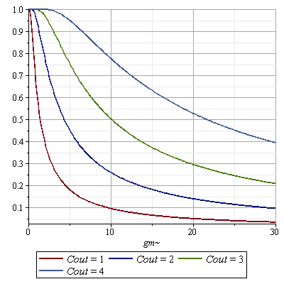
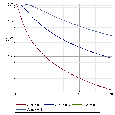
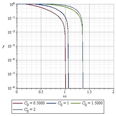
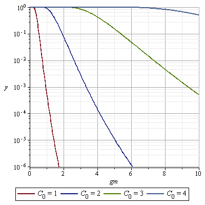
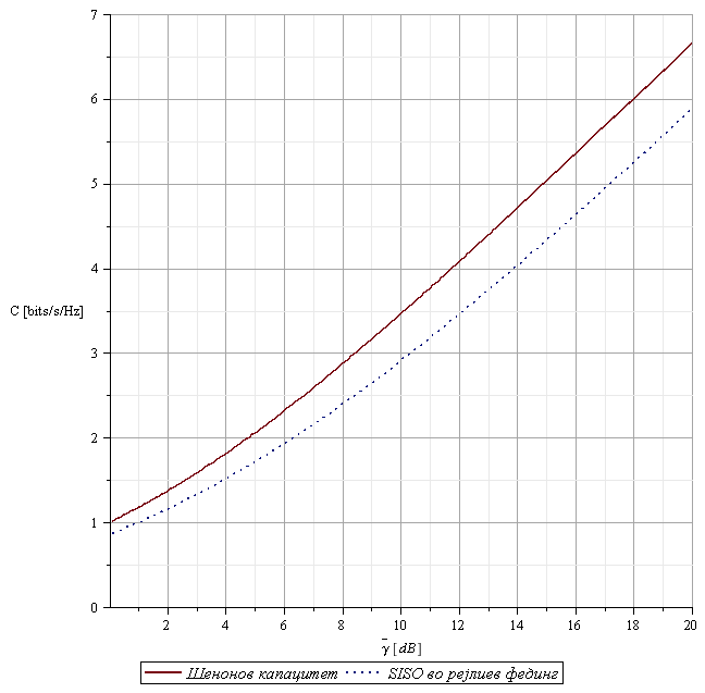

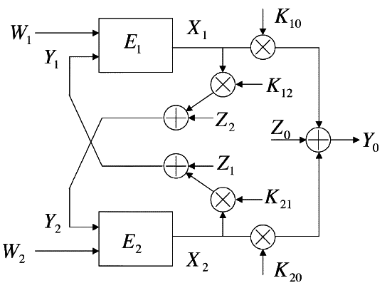
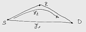
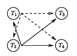
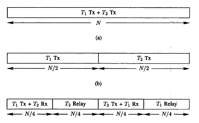
.png)