\sloppy
Paper- T.Cover, Capacity theorem for the Relay Channels
Abstract- Relay channel consist of an input x1, a relay output y1, a channel output y , and a relay sender x2 (whose transmission is allowed to depend on the past symbols y1). The dependence of the received symbols upon the inputs is given by p(y, y1|x1, x2). The channel is assumed to be memoryless. In this paper following capacity theorems are proved.
1. If y is a degraded form of y1, then
C = maxp(x1, x2)min{I(X1, X2;Y), I(X1;Y1|X2)}.
2. If
y1 is degraded form of
y, then
C = maxp(x1)maxx2{I(X1;Y|x2).
3. If
p(y, y1|x1, x2) is an
arbitrary relay channel with feedback from
(y, y1) to both
x1 and
x2, then
C = maxp(x1, x2)min{I(X1, X2;Y), I(X1; Y, Y1|X2)}
4. For a general relay channel
\mathchoiceC ≤ maxp(x1, x2)minI(X1, X2;Y), I(X1;Y, Y1|X2)C ≤ maxp(x1, x2)minI(X1, X2;Y), I(X1;Y, Y1|X2)C ≤ maxp(x1, x2)minI(X1, X2;Y), I(X1;Y, Y1|X2)C ≤ maxp(x1, x2)minI(X1, X2;Y), I(X1;Y, Y1|X2)
Од овој израз може да сконташ дека капацитетот на генерален рејлиев канал е аналоген на max-flow min-cut алгоритамот. Го сконтав откако ја помина вглавата 15.7 од EIT.
Во EIT книгата наместо X2 користат X1, а наместо X1 користат X. Таму кпацитетот на генерален рејлиев канал е:
C ≤ supp(x, x1)min{I(X, X1;Y), I(X;Y, Y1|X1)}
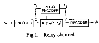
1 Introduction
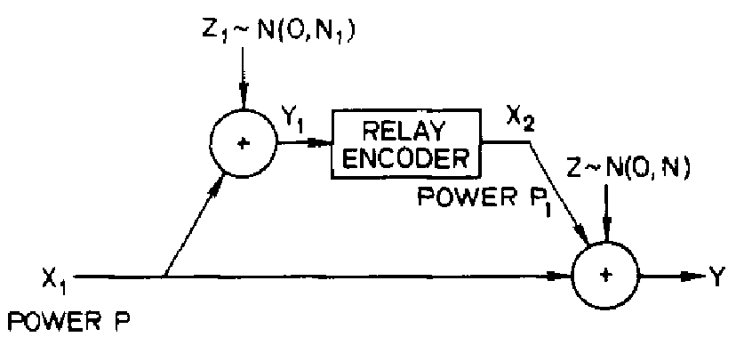
THE Discrete memoryless relay channel denoted as
(X1x X2 , p(y, y1|x1, x2), YxY2) consist of four finite sets:
X\mathnormal1, X\mathnormal2, Y, Y\mathnormal1 and a collection of probability distributions
p(., .|x1, x2) on
YxY\mathnormal1one for each
(x1, x2) ∈ X\mathnormal1xX\mathnormal2. The interpretation is that
x1 is the input to the channel and
y is the output,
y1 is the relay output and
x2 is the input symbol chosen by the relay as shown on
1↑. The channel is memoryless in the sense that the current received symbols
(Yi2, Yi3) and the message and past symbols
(m, Xi−11, Xi−12, Yi−12, Yi−13) are conditionally independent given the current transmitted symbols
(Xi1, Xi2). The problem is to find the capacity of the channel between the sender
x1 and the receiver
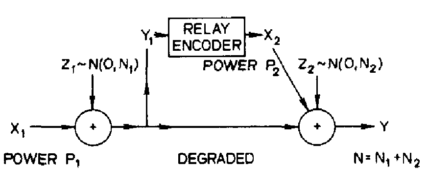
y. The model that motivates our investigation of degraded relay channels is perhaps best illustrated in the Gaussian case (
4↓). Suppose the transmitter
x1 has power
P1 and the relay transmitter has power
P2. The relay receiver
\mathchoicey1y1y1y1 sees
\mathchoicex1 + z1x1 + z1x1 + z1x1 + z1,
z1 = N(0, N1). The intended receiver
y sees the sum of the relay signal
x2 and a corrupted version of y1, i.e.,
y = x2 + y1 + z2 z2 ~ N(0, N2).
How should x2 use his knowledge of x1 (obtained through y1) to help y understand x1?
За да сватиш зошто се вакви ознаките треба да го видиш чланакот од van der Meulen
We shell show that capacity is given with
C* = max0 ≤ α ≤ 1min⎧⎩C⎛⎝⎛⎝(P1 + P2 + 2√( α⋅P1P2))/(N1 + N2)⎞⎠, C⎛⎝(αP)/(N1)⎞⎠⎞⎠⎫⎭
where C(x) = (1)/(2)log(1 + x). An interpretation consistent with achieving C* in this example is that y1 discovers x1 perfectly, then x2 and x1 cooperate coherently in the next block to resolve the remaining y uncertainty about x1.
Многу убаво кажано H(x1|y) неизвесност колку добро го знаеш x1 ако го знеш y
However, in this next block, fresh x1 information is superimposed, thus resulting in a steady-state resolution of the past uncertainty and infusion of new information.
An (M, n) code for the relay channel consist of a set of integers:
a set of relay functions
{fi}ni = 1 such that:
Дефиницијата на симболот што се испраќа одговара на дефиницијата на стратегиите во релето во чланакот од van der Meulen. Со други зборови овде сака да каже дека сигналот што го испраќа релето во i-от тајмслот зависи од (i − 1)-те претходно примените сигнали во релето.
For generality, the encoding functions x1(⋅), fi(⋅) and decoding function g(⋅) are allowed to be stochastic functions.
Note that the allowed relay encoding functions actually form part of the definition o the relay channel because of the non-anticipatory relay condition. The relay channel input x2i is allowed to depend only on the past \mathchoiceyi1 = (y11, yi1, …, y1 i − 1)yi1 = (y11, yi1, …, y1 i − 1)yi1 = (y11, yi1, …, y1 i − 1)yi1 = (y11, yi1, …, y1 i − 1). The channel is memory-less in the sense that (yi, y1 i) depends on the past (xi1, xi2) only through the current transmitted symbols (x1 i, x2 i). Thus, for any choice p(w), w ∈ M, and code choice x1: W → X\mathnormaln\mathnormal1 and relay functions {fi}ni = 1, the joint probability mass function on W\mathnormalxX\mathnormaln\mathnormal1\mathnormalxX\mathnormaln\mathnormal2\mathnormalxY\mathnormaln\mathnormalxY\mathnormaln\mathnormal1 is given by:
n = 2
p(w, x1, x2, y, y1) = p(w)∏2i = 1p(x1i|w)p(x2i|y11, y12, …, y1i − 1)⋅p(yi, y1i|x1i, x2i)
= p(w)⋅p(x11|w)p(x21)⋅p(y1, y11|x11, x21)p(x12|w)p(x22|y11)⋅p(y2, y12|x12, x22)
Сака да каже: X1 зависи од W, X2 зависи од Y1 a (Y, Y1) зависат од (X1, X2)
If the message
w ∈ W is sent, let
Потсетување од EIT на Cover
λ(w) = Pr(g(Yn) ≠ w|Xn = xn(w)) = ⎲⎳ynP(yn|xn(w))⋅I(g(yn) ≠ w)
denote the conditional probability of error. We define the average probability of error of the code to be:
The probability of error is calculated under a special distribution - uniform distribution over the codewords w ∈ [1, M]. Finally let:
be the maximal probability of error for the (M, n) code.
The rate R of an (M, n) code is defined by:
The rate R is said to be achievable by a relay channel if, for any ϵ > 0 and for all n sufficiently large, there exist an (M, n)code with
R − ϵ ≤ (1)/(n)⋅log(M); n⋅(R − ϵ) ≤ log(M); 2n⋅(R − ϵ) ≤ M
such as that λn ≤ ϵ. The capacity C of the relay channel is the supremum of the set of achievable rates.
мое прво резонирање:
log(M) ≥ nR; R ≤ (1)/(n)⋅log(M)
(This is bit different definition of achievability compared to the definition in the T. Cover textbook.)
Кога го преведував за докторатот, ми стана логичен на крај изразот
9↑. Се сетив на noisy typewriter. Таму дактилографката ја греши секоја втора буква.
M = 28 а
R = log(14)
M ≥ 2log(14) = 14. Значи ако имаш безгрешна дактилографка тогаш M = 28 = 2log(|X|) = 2log(28).
We now consider a family of relay channels in which the relay receiver y1 is better than the ultimate receiver y in the sense defined below.
Definition(degraded): (current)
The relay channel
(X\mathnormal1xX\mathnormal2, \mathnormalp(y, y1|x1, x2), YxY\mathnormal1) is said to be
degraded if
p(y, y1|x1, x2) can be written in the form
Equivalently, we see by inspection of
10↑ that a relay channel is degraded if
p(y|x1, x2, y1) = p(y|x2, y1) i.e.,
\mathchoiceX1 → (X2, Y1) → YX1 → (X2, Y1) → YX1 → (X2, Y1) → YX1 → (X2, Y1) → Y form Markov chain
.
Дефиницијата сака да каже дека за дадени x2 i y1, y не зависи од x1.
p(X, Z|Y) = (p(X, Y, Z))/(P(Y)) = (p(X, Y)⋅p(Z|X, Y))/(P(Y)) = (p(X, Y)⋅p(Z|Y))/(P(Y)) = p(X|Y)⋅p(Z|Y) (ова ако добро се сеќавам е дефинција за Markov chain X → Y → Z)
The previously discussed Gaussian channel is therefore degraded. For the reader familiar with the definition of the degraded broadcast channel, we observe that a degraded relay channel can be looked at as a family of physically degraded broadcast channels indexed by x2. A weaker form of degradation (stochastic) can be defined for relay channels, but Theorem 1 below then becomes only an inner bound to the capacity. The case in which the relay y1 is worse than y is less interesting (except for the converse) and is defined as follows.
Сака да каже дека во нормални услови сигналот во релето y1 е подобар од сигналот во приемникот. За обратно деградиран канал сигналот во приемникот е подобар од сигналот во релето.
Definition: (reversely degraded):
The relay channel
(X\mathnormal1xX\mathnormal2, \mathnormalp(y, y1|x1, x2), YxY\mathnormal1) is
reversely degraded if
p(y, y1|x1, x2) can be written in following form
The main contribution of this paper is summarized by the following three theorems.
Theorem 1:(degraded relay channel)
The capacity
C of the
degraded relay channel is given
where supremum is over all joint distributions p(x1, x2) on (X\mathnormal1, X\mathnormal2).
Theorem 2:(reversely degraded relay channel)
The capacity
C0 of the
reversely degraded relay channel is given by
Theorem 2 has a simple interpretation. Since the relay y1 sees a corrupted version of what y sees, x2 can contribute no new information to y - thus x2 is set constantly at the symbol that „opens“ the channel for the transmission of x1 directly to y at rate I(X1;Y|x2). The converse proves that one can do no better.
Theorem 1 has a more interesting interpretation. The first term in the brackets in
12↑ sugest that a rate
I(X1, X2;Y) can be achieved where
p(x1, x2) is arbitrary. However, this rate can only be achieved by complete cooperation of
x1 and
x2.
To set up this cooperation x2 must know x1. Thus the
x1 rate of transmission should be less than
I(X1;Y1|X2). (How they cooperate given these two conditions will be left to the proof.) Finally, both constraints lead to the minimum characterization in
12↑.
I(X1, X2;Y)
= \cancelto0 − x2can contribute no new information to y I(X2;Y1) + I(X1;Y1|X2) = I(X1;Y1) + I(X2;Y1|X1); I(X1, X2;Y) ≥ I(X1;Y1|X2)
I(X2;Y1|X1)
= H(X2|X1) − H(Y1|X1, X2) = − H(Y1|X1)
Сака да каже ако x2 може да придонесе со нова информација на y тогаш \strikeout off\uuline off\uwave offI(X1, X2;Y) ≥ I(X1;Y1|X2) ако не придонесува нова информација тогаш\uuline default\uwave default \strikeout off\uuline off\uwave offI(X1, X2;Y)=I(X1;Y1|X2)
\strikeout off\uuline off\uwave offКоја е поентата тогаш да зема минимум?
18.06.14
I(X1, X2;Y) = \overset(*)I(X2;Y1) + I(X1;Y1|X2) = I(X1;Y1) + I(X2;Y1|X1); I(X1, X2;Y) ≥ I(X1;Y1|X2)
(*) - Мислам дека овој член е 0 зошто X2 е функција од Y1.
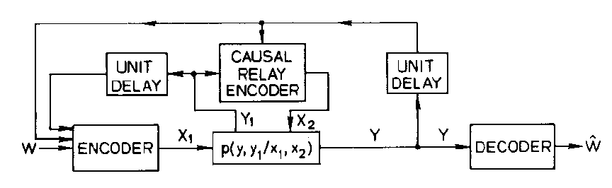
The obvious notion of an arbitrary relay channel with causal feedback (from both y and y1 to x1 and x2) will be formalized in Section V. The following theorem can then be proved.
Theorem 3:(arbitrary channel)
The Capacity of
CFB of an
arbitrary relay channel with feedback is given by:
Note that CFB is the same as C except that Y1 is replaced by (Y, Y1) in I(X1;Y1|X2). The reason is that the feedback changes an arbitrary relay channel into a degraded relay channel in which x1 transmits information to x2 by way of y1 and y. Clearly Y is a degraded form of (Y, Y1).
Theorem 2 is included for reasons of completeness, but it can be shown to follow from a chain of remarks in
[1] under slightly stronger conditions. Specifically in
[1] .
R1 = C1(1, 2),
\mathchoiceLema4.1.Lema4.1.Lema4.1.Lema4.1. C1(1, 3) ≤ C1[1, (2, 3)] with equality if both
P(y2, y3|x1x2x3) = P(y2|x1, x2, x3)P(y3|x1, x2, x3)
(i.e., the outputs y2 and y3 are conditionally independent given the inputs x1x2 and x3, and \mathchoiceC1(1, 2) = 0C1(1, 2) = 0C1(1, 2) = 0C1(1, 2) = 0.
\strikeout off\uuline off\uwave off\mathchoiceTheorem 10.1.Theorem 10.1.Theorem 10.1.Theorem 10.1. \uuline default\uwave defaultFor any n a (1, 3)-code (n, M, λ) satisfies
logM ≤ (n⋅U + 1)/(1 − λ)
\mathchoiceTheorem7.1.Theorem7.1.Theorem7.1.Theorem7.1.Let
ϵ > 0 and
0 < λ ≤ 1 be arbitrary. For any d.m. three-terminal channel and all
n sufficiently large there exists a
(1, 3) -code
(n, M, λ) with
M > 2n[C(1, 3) − ϵ].
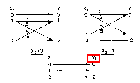
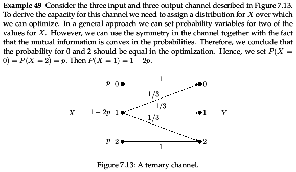
Before proving the theorems, we apply the result
12↑ to a
simple example introduced by Sato
[4]. The channel as shown in
2↑ has
X\mathnormal1 = Y = Y\mathnormal1 = \mathnormal\mathnormal\mathnormal{0, 1, 2},
X\mathnormal2 = \mathnormal{0, 1}, and the conditional probability
p(y, y1|x1, x2) satisfies
10↑. Specifically, the channel operation is:
and
p(y|y1, x2 = 0) =
y1 = 0
y1 = 1
y1 = 2
\overset
y = 0
y = 1
y = 2
⎡⎢⎢⎢⎣
1
0
0
0
0.5
0.5
0
0.5
0.5
⎤⎥⎥⎥⎦
Sato calculated a cooperative upper bound to the channel capacity of the channel, \mathchoiceRUG = maxp(x1, x2)I(X1, X2;Y) = 1.170RUG = maxp(x1, x2)I(X1, X2;Y) = 1.170RUG = maxp(x1, x2)I(X1, X2;Y) = 1.170RUG = maxp(x1, x2)I(X1, X2;Y) = 1.170.
By restricting the relay encoding functions to
i)
x2i = f(y11, ..., y1i − 1) = f(y1i − 1)
1 < i ≤ n,
ii)
x2i = f(y11, ..., y1i − 1) = f((y1i − 2, y1i − 1)
1 < i ≤ n.
Sato calculated two lower bounds to the capacity of the channel:
i)
R1 = 1.0437
ii)
R2 = 1.0549
From Theorem 1 we obtain the true capacity C = 1.161878. The optimal joint distribution on X\mathnormal1xX\mathnormal2 is given in Table 1.
We shall see that instead of letting the encoding functions of the relay depend only on a finite number of previous
y1 transmissions, we can achieve
C by allowing
block Markovian dependence of x2 and y1 in a manner similar to
[6].
Од El Gamal NIT:
Since the relay codeword transmitted in a block depends statistically on the message transmited in the previous block, we reffer to this scheme as block Markov coding (BMC)
Подолу се обидите да го добијам C = 1.161878. Го добив во последниот обид 5↓. Пресметувам само I(X1, X2;Y) но не и I(X1;Y1|X2). Исто така сеуште не успеав да ја добијам сам оптималната дистрибуција од чланакот но ја добив 5↓ дистрибуцијата од NIT Lecture Notes Relay with limmited lookahead (која претходно ја проверував во 5↓). Тоа е таа дистрибуција од која Cover го добива RUG = maxp(x1, x2)I(X1, X2;Y).
02.07.14
Сега ми текна дека дистрибуцијата од чланакот ја имаат добиено со Lagrange Multipliers. Така немам пробано. Само легитимен ми е начинот со извод и не знам зошто би пробувал на дру начин.
04.07.14
Ова од 02.07 мислам дека не треба да се проверува. C = 1.161878 се добива со рестрикција на кодирачката функција да зависи од еден претходен симбол но не и порака. Не знам како се прави сега тоа. Веројатно треба да работам со n-битни низи. Засега ќе го оставам на on-hold.
Не, не, не!!! C = 1.161878 е true capacity изгледа треба да го пресметам I(X1;Y1Y|X2). Јас цело време се мотав пресметувајќи го I(X1;Y1|X2) а тоа е за деградиран релеен канал.
C = maxp(x1, x2)I(X1, X2;Y); I(X1, X2;Y) = H(Y) − H(Y|X1, X2) = H(X1, X2) − H(X1, X2|Y)H(Y|X2 = 0) = ∑xp(x1)⋅H(Y|X2 = 0, X1 = x1) = p(X1 = 0)⋅H(Y|X2 = 0, X1 = 0) + p(X1 = 1)⋅H(Y|X2 = 0, X1 = 1) + p(X1 = 2)⋅H(Y|X2 = 0, X1 = 2)
H(Y|X2 = 0, X1) = ∑x1p(x1)⋅H(Y|X2 = 0, X1 = x1) = p(X1 = 0)⋅0 + p(x1 = 1)⋅[ − p(Y = 1|X2 = 0, X1 = 1)⋅log(p(Y = 1|X2 = 0, X1 = 1)) − p(Y = 2|X2 = 0, X1 = 1)⋅log(p(Y = 2|X2 = 0, X1 = 1))] + p(X1 = 2)⋅[ − p(Y = 1|X2 = 0, X1 = 2)⋅log(p(Y = 1|X2 = 0, X1 = 2) − p(Y = 2|X2 = 0, X1 = 2)⋅log(p(Y = 2|X2 = 0, X1 = 2))] = 0 + p(X1 = 1)⋅1 + p(X1 = 2)⋅1
H(Y|X2 = 1, X1) = ∑x1p(x1)⋅H(Y|X2 = 1, X1 = x1) = p(X1 = 2)⋅0 + p(X1 = 0)⋅( − p(Y = 0|X2 = 1, X1 = 0)⋅log(p(Y = 0|X2 = 1, X1 = 0) − p(Y = 1|X2 = 1, X1 = 0)⋅log(p(Y = 1|X2 = 1, X1 = 0)) + p(X1 = 1)⋅( − p(Y = 1|X2 = 1, X1 = 1)⋅log(p(Y = 1|X2 = 1, X1 = 1) − p(Y = 0|X2 = 1, X1 = 1)⋅log(p(Y = 0|X2 = 1, X1 = 1)) = 0 + p(X1 = 0)⋅1 + p(X1 = 1)⋅1
\strikeout off\uuline off\uwave offH(Y|X1, X2) = ∑x2p(x2)⋅H(Y|X1, X2 = x2) = p(X2 = 0)⋅H(Y|X2 = 0, X1) + p(X2 = 1)⋅H(Y|X2 = 1, X1) =
= \mathchoicep(X2 = 0)⋅(p(X1 = 1) + p(X1 = 2)) + p(X2 = 1)⋅(p(X1 = 0) + p(X1 = 1))p(X2 = 0)⋅(p(X1 = 1) + p(X1 = 2)) + p(X2 = 1)⋅(p(X1 = 0) + p(X1 = 1))p(X2 = 0)⋅(p(X1 = 1) + p(X1 = 2)) + p(X2 = 1)⋅(p(X1 = 0) + p(X1 = 1))p(X2 = 0)⋅(p(X1 = 1) + p(X1 = 2)) + p(X2 = 1)⋅(p(X1 = 0) + p(X1 = 1))
\strikeout off\uuline off\uwave offI(X1, X2;Y) = H(Y) − (p(X2 = 0)⋅p(X1 = 1) + p(X2 = 0)⋅p(X1 = 2) + p(X2 = 1)⋅p(X1 = 0) + p(X2 = 1)⋅p(X1 = 1))
\strikeout off\uuline off\uwave offC = log(3) − H(Y|X1, X2) = log(3) − (p(X2 = 0)⋅p(X1 = 1) + p(X2 = 0)⋅p(X1 = 2) + p(X2 = 1)⋅p(X1 = 0) + p(X2 = 1)⋅p(X1 = 1)) = \normalcolor1.2935825010
\strikeout off\uuline off\uwave off
Ова последново во е согласно веројатностите дадени во чланакот
\strikeout off\uuline off\uwave off
x2 = 0
x2 = 1
\overset
x1 = 0
x2 = 1
x3 = 2
⎡⎢⎣
0.35431
0.072845
0.072845
0.072845
0.072845
0.35431
⎤⎥⎦
\strikeout off\uuline off\uwave offp(X2 = 0)⋅p(X1 = 1) + p(X2 = 0)⋅p(X1 = 2) + p(X2 = 1)⋅p(X1 = 0) + p(X2 = 1)⋅p(X1 = 1) = p(x2 = 0, x1 = 1) + p(02) + p(10) + p(11) = 0.2913800000
0.072845 + 0.072845 + 0.072845 + 0.072845 = 0.29138
\strikeout off\uuline off\uwave off
H(Y|X1, X2) = ∑x1, x2p(x1, x2)⋅H(Y|X2 = x2, X1 = x1) = p(0, 0)H(Y|00) + p(01)H(Y|01) + p(0, 2)H(Y|02) + p(1, 0)H(Y|10) + p(11)H(Y|11) + p(1, 2)H(Y|12)
H(Y|00) = H(Y|X2 = 0, X1 = 0) = 0; H(Y|01) = 1; H(Y|02) = 1H(Y|10) = H(Y|X2 = 1, X1 = 0) = 1; H(Y|11) = 1; H(Y|12) = 0
\strikeout off\uuline off\uwave offH(Y|X1, X2) = ∑x1, x2p(x1, x2)⋅H(Y|X2 = x2, X1 = x1) = 0 + 0.072845⋅1 + 0.072845⋅1 + 0.072845⋅1 + 0.072845⋅1 + 0 = 0.2913800000
log2(3) − H(Y|X1,X2) = 1.585 − 0.2913800000 = 1.29362
И на овој начин пак го добивам истиот капацитет
Мојот резултат
5↑ не одговара на резултатот од чланакот. Мислам дека лошо го рачунам
H(Y) !?
Дали можеби треба вака:
log3(3) − H(Y|X1,X2) = 1 − 0.2913800000 = 0.70862 ternary symbols/transmission
(0.70862)/(log3(2)) = 1.123136127 bits/transmission
x = logm(y) mx = y ⁄ log2(...) x⋅log2(m) = log2(y) x = (log2(y))/(log2(m)) logm(y) = (log2(y))/(log2(m))
x = log2(y) 2x = y ⁄ logm(...) x⋅logm(2) = logm(y) x = (logm(y))/(logm(2)) log2(y) = (logm(y))/(logm(2))
Ова е втор обид откако го поминав чланакот од van der Meulen
p(y|x1, x2 = 0) =
x1 = 0
x1 = 1
x1 = 2
\overset
y = 0
y = 1
y = 2
⎡⎢⎢⎢⎣
1
0
0
0
0.5
0.5
0
0.5
0.5
⎤⎥⎥⎥⎦
p(y|x1, x2 = 1) =
x1 = 0
x1 = 1
x1 = 2
\overset
y = 0
y = 1
y = 2
⎡⎢⎢⎢⎣
0.5
0.5
0
0.5
0.5
0
0
0
1
⎤⎥⎥⎥⎦
y1 ≡ x1
I(X1, X2;Y) = H(Y) − H(Y|X1, X2) = H(X1, X2) − H(X1, X2|Y)
H(Y|X1X2) = P(X2 = 0)⋅H(Y|X1X2 = 0) + P(X2 = 1)⋅H(Y|X1X2 = 1)
H(Y|X1X2 = 0) = p(X1 = 0)⋅H(Y|X1 = 0, X2 = 0) + p(X1 = 1)⋅H(Y|X1 = 1, X2 = 0) + p(X1 = 2)⋅H(Y|X1 = 2, X2 = 0) = p(X1 = 1) + p(X1 = 2)
H(Y|X1X2 = 1) = p(X1 = 0)⋅H(Y|X1 = 0, X2 = 1) + p(X1 = 1)⋅H(Y|X1 = 1, X2 = 1) + p(X1 = 2)⋅H(Y|X1 = 2, X2 = 1) = p(X1 = 0) + p(X1 = 1)
\strikeout off\uuline off\uwave offH(Y|X1X2) = P(X2 = 0)⋅H(Y|X1X2 = 0) + P(X2 = 1)⋅H(Y|X1X2 = 1) = P(X2 = 0)[p(X1 = 1) + p(X1 = 2)] + P(X2 = 1)⋅[p(X1 = 0) + p(X1 = 1)]
I(X1, X2;Y) = H(Y) − H(Y|X1, X2) = H(Y) − p(X2 = 0)⋅[p(X1 = 1) + p(X1 = 2)] − P(X2 = 1)⋅[p(X1 = 0) + p(X1 = 1)]
= H(Y) − p(X1 = 1) − (X2 = 0)⋅p(X1 = 2) + P(X2 = 1)⋅p(X1 = 0)
log2(3) = 1.585 − − 1 ⁄ 3 − 1 ⁄ 2⋅1 ⁄ 3 − 1 ⁄ 2⋅1 ⁄ 3 = 1.585 − (2)/(3) = 1.585 − 0.67 = 0.918 ternary symbols/transmission
(0.918)/(log2[3]) = 0.5791 bits/transmission
\strikeout off\uuline off\uwave offI(X1;Y1|X2) = H(Y1) − H(Y1|X1X2) = log2(3) зошто x1 ≡ y1
I(X1, X2;Y) ≥ I(X1;Y1|X2)
Ако одам со оптималните вредности за веројатноста од чланакот
\strikeout off\uuline off\uwave off
x2 = 0
x2 = 1
\overset
x1 = 0
x2 = 1
x3 = 2
⎡⎢⎣
0.35431
0.072845
0.072845
0.072845
0.072845
0.35431
⎤⎥⎦
I(X1, X2;Y)
= H(Y) − H(Y|X1, X2) = H(Y) − (X2 = 0)⋅[p(X1 = 1) + p(X1 = 2)] − P(X2 = 1)⋅[p(X1 = 0) + p(X1 = 1)] =
\mathchoiceH(Y) − p(X2 = 0)⋅p(X1 = 1) − p(X2 = 0)⋅p(X1 = 2) − p(X2 = 1)⋅p(X1 = 0) − p(X2 = 1)⋅p(X1 = 1) = H(Y) − p(X2 = 0)⋅p(X1 = 1) − p(X2 = 0)⋅p(X1 = 2) − p(X2 = 1)⋅p(X1 = 0) − p(X2 = 1)⋅p(X1 = 1) = H(Y) − p(X2 = 0)⋅p(X1 = 1) − p(X2 = 0)⋅p(X1 = 2) − p(X2 = 1)⋅p(X1 = 0) − p(X2 = 1)⋅p(X1 = 1) = H(Y) − p(X2 = 0)⋅p(X1 = 1) − p(X2 = 0)⋅p(X1 = 2) − p(X2 = 1)⋅p(X1 = 0) − p(X2 = 1)⋅p(X1 = 1) =
log2(3) − p(01) − p(02) − p(10) − p(11) = log2(3) − 4⋅0.072845 = 0.585 − 0.2913800000 = 1.29362
p(10) + p(20) + p(01) + p(11)
Сега сакам да го пресметам
H(Y) како што треба:
p(Y = 0|X2 = 0) = p(X1 = 0) = p10; p(Y = 1|X2 = 0) = (p(X1 = 1))/(2) + (p(X1 = 2))/(2) = (p11)/(2) + (p12)/(2); p(Y = 2|X2 = 0) = (p11)/(2) + (p12)/(2) пази индексот „12“ одговара на x1 = 2
p(Y = 0|X2 = 1) = (p(X1 = 0))/(2) + (p(X1 = 1))/(2) = (p10)/(2) + (p11)/(2); p(Y = 1|X2 = 1) = (p(X1 = 0))/(2) + (p(X1 = 1))/(2) = (p10)/(2) + (p11)/(2); p(Y = 2|X2 = 1) = p(X1 = 2) = p12;
p(Y = 0) = p20⋅p10 + p21⎛⎝(p10 + p11)/(2)⎞⎠; p(Y = 1) = p20⋅(p11 + p12)/(2) + p21⋅(p10 + p12)/(2); p(Y = 2) = p20⋅(p11 + p12)/(2) + p21⋅p12
Ова во квадратчево не е добро требa да биде p11.
А̀ко земам дека
p20 = p21 = (1)/(2)
p(Y = 0) = (p10)/(2) + (1)/(2)⋅⎛⎝(p10 + p11)/(2)⎞⎠ = (3p10)/(4) + (p11)/(4); p(Y = 1) = (1)/(2)⋅(p11 + p12)/(2) + (1)/(2)⋅(p10 + p11)/(2) = (p10)/(4) + (p11)/(2) + (p12)/(4); p(Y = 2) = (1)/(2)⋅(p11 + p12)/(2) + (p12)/(2) = (p11)/(4) + (3⋅p12)/(4)
− H(Y) = p(Y = 0)⋅log(p(Y = 0)) + p(Y = 1)⋅log(p(Y = 1)) + p(Y = 2)⋅log(p(Y = 2))
H(Y) = H⎛⎝(3⋅p10 + p11)/(4), (p10 + 2⋅p11 + p12)/(4), (p11 + 3⋅p12)/(4)⎞⎠
− H(Y) = (3⋅p10 + p11)/(4)⋅log⎛⎝(3⋅p10 + p11)/(4)⎞⎠ + (p10 + 2⋅p11 + p12)/(4)⋅log⎛⎝(p10 + 2⋅p11 + p12)/(4)⎞⎠ + (p11 + 3⋅p12)/(4)⋅log⎛⎝(p11 + 3⋅p12)/(4)⎞⎠
\strikeout off\uuline off\uwave offH(Y) = (3⋅p10 + p11)/(4)⋅log⎛⎝(3⋅p10 + p11)/(4)⎞⎠ + (p10 + 2⋅p11 + 1 − p10 − p11)/(4)⋅log⎛⎝(p10 + 2⋅p11 + 1 − p10 − p11)/(4)⎞⎠ + (p11 + 3⋅(1 − p10 − p11))/(4)⋅log⎛⎝(p11 + 3⋅(1 − p10 − p11))/(4)⎞⎠
H(Y) = (3⋅p10 + p11)/(4)⋅log⎛⎝(3⋅p10 + p11)/(4)⎞⎠ + (p11 + 1)/(4)⋅log⎛⎝(p11 + 1)/(4)⎞⎠ + (p11 + 3 − 3p10 − 3p11)/(4)⋅log⎛⎝(p11 + 3 − 3p10 − 3p11)/(4)⎞⎠
H(Y) = (3⋅p10 + p11)/(4)⋅log⎛⎝(3⋅p10 + p11)/(4)⎞⎠ + (p11 + 1)/(4)⋅log⎛⎝(p11 + 1)/(4)⎞⎠ + (3 − 3⋅p10 − 2⋅p11)/(4)⋅log⎛⎝(3 − 3⋅p10 − 2⋅p11)/(4)⎞⎠
Ако земам
5↑ тогаш со изводи во мапле најдов дека
H(Y) = log2(3).
Треба да се реши со произволни вредности на p20, p21. Го решив во maple ама пак добив дека H(Y) = log(3). Кога барав извод од изразот во магента не добивав резултат.
-
Треба да се реши каде p(x1) и p(x2) нема да ги третирам независно туку каде ќе зависат еден од друг т.е. да го претставам I(...) преку здружените веројатностиp(x1, x2) па потоа да вадам извод по p(x1, x2) .
p(y|x1, x2 = 0) =
x1 = 0
x1 = 1
x1 = 2
\overset
y = 0
y = 1
y = 2
⎡⎢⎢⎢⎣
1
0
0
0
0.5
0.5
0
0.5
0.5
⎤⎥⎥⎥⎦
p(y|x1, x2 = 1) =
x1 = 0
x1 = 1
x1 = 2
\overset
y = 0
y = 1
y = 2
⎡⎢⎢⎢⎣
0.5
0.5
0
0.5
0.5
0
0
0
1
⎤⎥⎥⎥⎦
p(x2) = 0; ⎡⎢⎢⎢⎣
p(y0)
p(y1)
p(y2)
⎤⎥⎥⎥⎦ = ⎡⎢⎢⎢⎣
1
0
0
0
0.5
0.5
0
0.5
0.5
⎤⎥⎥⎥⎦⎡⎢⎢⎢⎣
p(x0)
p(x1)
p(x2)
⎤⎥⎥⎥⎦ p(x2) = 1; ⎡⎢⎢⎢⎣
p(y0)
p(y1)
p(y2)
⎤⎥⎥⎥⎦ = ⎡⎢⎢⎢⎣
0.5
0.5
0
0.5
0.5
0
0
0
1
⎤⎥⎥⎥⎦⎡⎢⎢⎢⎣
p(x0)
p(x1)
p(x2)
⎤⎥⎥⎥⎦
\strikeout off\uuline off\uwave offH(Y|X1, X2) = ∑x1, x2p(x1, x2)⋅H(Y|X2 = x2, X1 = x1) = p(0, 0)H(Y|00) + p(10)H(Y|10) + p(20)H(Y|20) + p(01)H(Y|01) + p(11)H(Y|11) + p(2, 1)H(Y|21)
= p(00)⋅0 + \mathchoicep(10) + p(20) + p(01) + p(11)p(10) + p(20) + p(01) + p(11)p(10) + p(20) + p(01) + p(11)p(10) + p(20) + p(01) + p(11) + p(21)⋅0 го имав p(11) пропуштено!!!
Пази на индексите овде се разликуваат од индексите кога ги пресметував условните веројатности погоре. На пример овде „20” подразбира x1 = 2, x2 = 0
Подолниве изрази за p(Y) се точни овие погоре немаат врска!!!
p(Y = 0) = p(X1 = 0, X2 = 0)⋅p(Y = 0|X1 = 0, X2 = 0) + p(X1 = 0, X2 = 1)⋅p(Y = 0|X1 = 0, X2 = 1) + p(X1 = 1, X2 = 1)⋅p(Y = 0|X1 = 1, X2 = 1) = \mathchoicep(00) + (p(01) + p(11))/(2);p(00) + (p(01) + p(11))/(2);p(00) + (p(01) + p(11))/(2);p(00) + (p(01) + p(11))/(2);
p(Y = 1) = \mathchoice(p(10) + p(20))/(2) + (p(01) + p(11))/(2)(p(10) + p(20))/(2) + (p(01) + p(11))/(2)(p(10) + p(20))/(2) + (p(01) + p(11))/(2)(p(10) + p(20))/(2) + (p(01) + p(11))/(2); p(Y = 2) = \mathchoice(p(10) + p(20))/(2) + p(21)(p(10) + p(20))/(2) + p(21)(p(10) + p(20))/(2) + p(21)(p(10) + p(20))/(2) + p(21)
H(Y) = − ⎛⎝p(00) + (p(01) + p(11))/(2)⎞⎠⋅log2⎛⎝p(00) + (p(01) + p(11))/(2)⎞⎠ − ⎛⎝(p(10) + p(20))/(2) + (p(01) + p(11))/(2)⎞⎠⋅log2⎛⎝(p(10) + p(20))/(2) + (p(01) + p(11))/(2)⎞⎠ − ⎛⎝(p(10) + p(20))/(2) + p(21)⎞⎠⋅log2⎛⎝(p(10) + p(20))/(2) + p(21)⎞⎠
p(00) + p(10) + p(20) + p(01) + p(11) + p(21) = 1 p(00) = 1 − p(10) + p(20) + p(01) + p(11) + p(21)
\strikeout off\uuline off\uwave off\mathchoicep(00) = a; p(10) = b; p(20) = c; p(01) = d; p(11) = e; p(21) = f;p(00) = a; p(10) = b; p(20) = c; p(01) = d; p(11) = e; p(21) = f;p(00) = a; p(10) = b; p(20) = c; p(01) = d; p(11) = e; p(21) = f;p(00) = a; p(10) = b; p(20) = c; p(01) = d; p(11) = e; p(21) = f;
\strikeout off\uuline off\uwave offa + b + c + d + e + f = 1
\strikeout off\uuline off\uwave offH(Y) = − ⎛⎝a + (d + e)/(2)⎞⎠⋅log2⎛⎝a + (d + e)/(2)⎞⎠ − ⎛⎝(b + c)/(2) + (d + e)/(2)⎞⎠⋅log2⎛⎝(b + c)/(2) + (d + e)/(2)⎞⎠ − ⎛⎝(b + c)/(2) + f⎞⎠⋅log2⎛⎝(b + c)/(2) + f⎞⎠
I(X1, X2;Y) = H(Y) − H(Y|X1X2) = − ⎛⎝a + (d + e)/(2)⎞⎠⋅log2⎛⎝a + (d + e)/(2)⎞⎠ − ⎛⎝(b + c)/(2) + (d + e)/(2)⎞⎠⋅log2⎛⎝(b + c)/(2) + (d + e)/(2)⎞⎠ − ⎛⎝(b + c)/(2) + f⎞⎠⋅log2⎛⎝(b + c)/(2) + f⎞⎠ − b − c − d − e
Можеби решението е:
\mathchoiceC = max(I(X1, X2;Y)) = log2(3) − b − c − d − e = log2(3) − 4⋅0.072845 = 1.2936C = max(I(X1, X2;Y)) = log2(3) − b − c − d − e = log2(3) − 4⋅0.072845 = 1.2936C = max(I(X1, X2;Y)) = log2(3) − b − c − d − e = log2(3) − 4⋅0.072845 = 1.2936C = max(I(X1, X2;Y)) = log2(3) − b − c − d − e = log2(3) − 4⋅0.072845 = 1.2936
\strikeout off\uuline off\uwave offC = supp(x1, x2)min{I(X1, X2;Y), I(X1;Y1|X2)}
После бара минимум. Може долната граница ја диктира: \strikeout off\uuline off\uwave offI(X1;Y1|X2) но како да го пресметам?
Со овој пристап и со претпоставка \mathchoiced + e = p(01) + p(11) = hd + e = p(01) + p(11) = hd + e = p(01) + p(11) = hd + e = p(01) + p(11) = h и \mathchoiceb + c = p(10) + p(20) = kb + c = p(10) + p(20) = kb + c = p(10) + p(20) = kb + c = p(10) + p(20) = k во мапле со парцијални изводи добив:
\mathchoice{a = 1 ⁄ 2 k, h = 2 ⁄ 3 − k, k = k}{a = 1 ⁄ 2 k, h = 2 ⁄ 3 − k, k = k}{a = 1 ⁄ 2 k, h = 2 ⁄ 3 − k, k = k}{a = 1 ⁄ 2 k, h = 2 ⁄ 3 − k, k = k}
\strikeout off\uuline off\uwave off
x2 = 0
x2 = 1
\overset
x1 = 0
x1 = 1
x1 = 2
⎡⎢⎣
0.35431
0.072845
0.072845
0.072845
0.072845
0.35431
⎤⎥⎦
\strikeout off\uuline off\uwave offp(00) = a = 0.35431 p(10) = b = 0.072845; p(20) = c = 0.072845; p(01) = d = 0.072845; p(11) = e = 0.072845; p(21) = f = 0.35431;
Ако го пресметам I(X1, X2;Y) за овие вредности се добива: I(X1, X2;Y) = 1.04256 што приближно одговара на R1 дадено подолу.
k = 2⋅0.072845 = 0.14569 h = 2 ⁄ 3 − 0.14569 = 0.52097666666667
h = 2⋅0.072845 = 0.14569 0.14569⋅2 = 0.29138
H(Y|X1, X2) = p(10) + p(20) + p(01) + p(11) = b + c + d + e
{a = 1 ⁄ 3 − 1 ⁄ 2 d − 1 ⁄ 2 e, b = 2 ⁄ 3 − c − d − e, d = d}
d = 0.072845
\strikeout off\uuline off\uwave offb = 2 ⁄ 3 − 0.072845 − 0.072845 − 0.072845 = 0.44813166666667
a = (1)/(2) − (0.072845)/(2) − (0.072845)/(2) = 0.26048833333333
{a = 4 ⁄ 9 − 1 ⁄ 2 d − 1 ⁄ 2 e, b = 2 ⁄ 9 − c − d − e, d = d}
a = 4 ⁄ 9 − 0.072845 ⁄ 2 − 0.072845 ⁄ 2 = 0.37159944444444
b = 2 ⁄ 9 − 0.072845 − 0.072845 − 0.072845 = 0.0036872222222222 0.0036872222222222⋅2 = 0.0073744444444444
Пример за ternary channel од Lund University скриптата
I(X;Y) = H(Y) − H(Y|X); H(Y|X) = p⋅H(Y|X = 0) + (1 − 2p)⋅H(Y|X = 1) + p⋅H(Y|X = 2) = (1 − 2p)log3(3)
− H(Y) = p(Y = 0)⋅log(p(Y = 0)) + p(Y = 1)⋅log(p(Y = 1)) + p(Y = 2)⋅log(p(Y = 2))
p(Y = 0) = (p + (1 − 2p)/(3)) = (1)/(3) + (p)/(3); p(Y = 1) = (1)/(3)⋅(1 − 2p) = (1)/(3) − (2p)/(3); p(Y = 2) = p + (1)/(3)⋅(1 − 2p) = (1)/(3) + (p)/(3);
H(Y) = H⎛⎝(1)/(3) + (p)/(3), (1)/(3) − (2p)/(3), (1)/(3) + (p)/(3)⎞⎠
\strikeout off\uuline off\uwave offI(X;Y) = H⎛⎝(1)/(3) + (p)/(3), (1)/(3) − (2p)/(3), (1)/(3) + (p)/(3)⎞⎠ − (1 − 2p)log3(3)
(d)/(dx)(I(X;Y)) = 0 → p0 = ...
После потстетувањето на проблемите од EIT 7.18 и 7.28
2C = 2C1 + 2C2 = 21 − H(p) + 20 = 3 ако p = 0 C = log2(3) = 1.585
C = log2(21 − H(p) + 1)
\strikeout off\uuline off\uwave off\mathchoiceC = log2⎡⎣exp2⎛⎝((1 − β)Hα + (α − 1)Hβ)/(β − α)⎞⎠ + exp2⎛⎝( − βHα + αHβ)/(β − α)⎞⎠⎤⎦C = log2⎡⎣exp2⎛⎝((1 − β)Hα + (α − 1)Hβ)/(β − α)⎞⎠ + exp2⎛⎝( − βHα + αHβ)/(β − α)⎞⎠⎤⎦C = log2⎡⎣exp2⎛⎝((1 − β)Hα + (α − 1)Hβ)/(β − α)⎞⎠ + exp2⎛⎝( − βHα + αHβ)/(β − α)⎞⎠⎤⎦C = log2⎡⎣exp2⎛⎝((1 − β)Hα + (α − 1)Hβ)/(β − α)⎞⎠ + exp2⎛⎝( − βHα + αHβ)/(β − α)⎞⎠⎤⎦
\strikeout off\uuline off\uwave off⎡⎢⎣
p(y0)
p(y1)
⎤⎥⎦ = ⎡⎢⎣
1
0
0.5
0.5
⎤⎥⎦⎡⎢⎣
p(x0)
p(x1)
⎤⎥⎦
Дефинитивно се работи за канал како оној во EIT 7.28
⎡⎢⎢⎢⎣
p(y0)
p(y1)
p(y2)
⎤⎥⎥⎥⎦ = ⎡⎢⎢⎢⎣
1
0
0
0
0.5
0.5
0
0.5
0.5
⎤⎥⎥⎥⎦⎡⎢⎢⎢⎣
p(x0)
p(x1)
p(x2)
⎤⎥⎥⎥⎦
2C = 21 − H(p) + 21 − H(q) = 21 − 0 + 21 − 1 = 2 + 1 = 3
C = log2(3) = 1.585
Theorem 3.3.3 од Ash не можеш да ја користиш зошто каналната матрица е сингуларна (проверив во Maple)!!!!
-
Се навраќам повторно на 5↑
p(y|x1, x2 = 0) =
x1 = 0
x1 = 1
x1 = 2
\overset
y = 0
y = 1
y = 2
⎡⎢⎢⎢⎣
1
0
0
0
0.5
0.5
0
0.5
0.5
⎤⎥⎥⎥⎦
p(y|x1, x2 = 1) =
x1 = 0
x1 = 1
x1 = 2
\overset
y = 0
y = 1
y = 2
⎡⎢⎢⎢⎣
0.5
0.5
0
0.5
0.5
0
0
0
1
⎤⎥⎥⎥⎦
p(x2) = 0; ⎡⎢⎢⎢⎣
p(y0)
p(y1)
p(y2)
⎤⎥⎥⎥⎦ = ⎡⎢⎢⎢⎣
1
0
0
0
0.5
0.5
0
0.5
0.5
⎤⎥⎥⎥⎦⎡⎢⎢⎢⎣
p(x0)
p(x1)
p(x2)
⎤⎥⎥⎥⎦ p(x2) = 1; ⎡⎢⎢⎢⎣
p(y0)
p(y1)
p(y2)
⎤⎥⎥⎥⎦ = ⎡⎢⎢⎢⎣
0.5
0.5
0
0.5
0.5
0
0
0
1
⎤⎥⎥⎥⎦⎡⎢⎢⎢⎣
p(x0)
p(x1)
p(x2)
⎤⎥⎥⎥⎦
p(y|x1x2)
y0
y1
y2
00
1
0
0
10
0
0.5
0.5
20
0
0.5
0.5
01
0.5
0.5
0
11
0.5
0.5
0
21
0
0
1
\strikeout off\uuline off\uwave offH(Y|X1, X2) = ∑x1, x2p(x1, x2)⋅H(Y|X2 = x2, X1 = x1) = p(0, 0)H(Y|00) + p(10)H(Y|10) + p(20)H(Y|20) + p(01)H(Y|01) + p(11)H(Y|11) + p(2, 1)H(Y|21)
= p(00)⋅0 + p(10) + p(20) + p(01) + p(11) + p(21)⋅0 го имав p(11) пропуштено!!!
p(Y = 0) = p(X1 = 0, X2 = 0)⋅p(Y = 0|X1 = 0, X2 = 0) + p(X1 = 0, X2 = 1)⋅p(Y = 0|X1 = 0, X2 = 1) + p(X1 = 1, X2 = 1)⋅p(Y = 0|X1 = 1, X2 = 1) = \mathchoicep(00) + (p(01) + p(11))/(2);p(00) + (p(01) + p(11))/(2);p(00) + (p(01) + p(11))/(2);p(00) + (p(01) + p(11))/(2);
p(Y = 1) = \mathchoice(p(10) + p(20))/(2) + (p(01) + p(11))/(2)(p(10) + p(20))/(2) + (p(01) + p(11))/(2)(p(10) + p(20))/(2) + (p(01) + p(11))/(2)(p(10) + p(20))/(2) + (p(01) + p(11))/(2); p(Y = 2) = \mathchoice(p(10) + p(20))/(2) + p(21)(p(10) + p(20))/(2) + p(21)(p(10) + p(20))/(2) + p(21)(p(10) + p(20))/(2) + p(21)
H(Y) = − ⎛⎝p(00) + (p(01) + p(11))/(2)⎞⎠⋅log2⎛⎝p(00) + (p(01) + p(11))/(2)⎞⎠ − ⎛⎝(p(10) + p(20))/(2) + (p(01) + p(11))/(2)⎞⎠⋅log2⎛⎝(p(10) + p(20))/(2) + (p(01) + p(11))/(2)⎞⎠ − ⎛⎝(p(10) + p(20))/(2) + p(21)⎞⎠⋅log2⎛⎝(p(10) + p(20))/(2) + p(21)⎞⎠
p(00) + p(10) + p(20) + p(01) + p(11) + p(21) = 1 p(00) = 1 − p(10) + p(20) + p(01) + p(11) + p(21)
\strikeout off\uuline off\uwave off\mathchoicep(00) = a; p(10) = b; p(20) = c; p(01) = d; p(11) = e; p(21) = f;p(00) = a; p(10) = b; p(20) = c; p(01) = d; p(11) = e; p(21) = f;p(00) = a; p(10) = b; p(20) = c; p(01) = d; p(11) = e; p(21) = f;p(00) = a; p(10) = b; p(20) = c; p(01) = d; p(11) = e; p(21) = f;
\strikeout off\uuline off\uwave offa + b + c + d + e + f = 1
\strikeout off\uuline off\uwave offH(Y) = − ⎛⎝a + (d + e)/(2)⎞⎠⋅log2⎛⎝a + (d + e)/(2)⎞⎠ − ⎛⎝(b + c)/(2) + (d + e)/(2)⎞⎠⋅log2⎛⎝(b + c)/(2) + (d + e)/(2)⎞⎠ − ⎛⎝(b + c)/(2) + f⎞⎠⋅log2⎛⎝(b + c)/(2) + f⎞⎠
\strikeout off\uuline off\uwave offH(Y|X1, X2) = p(10) + p(20) + p(01) + p(11) = b + c + d + e
I(X1, X2;Y) = − ⎛⎝a + (d + e)/(2)⎞⎠⋅log2⎛⎝a + (d + e)/(2)⎞⎠ − ⎛⎝(b + c)/(2) + (d + e)/(2)⎞⎠⋅log2⎛⎝(b + c)/(2) + (d + e)/(2)⎞⎠ − ⎛⎝(b + c)/(2) + f⎞⎠⋅log2⎛⎝(b + c)/(2) + f⎞⎠ − b − c − d − e
a = (4)/(9) − (d)/(2) − (e)/(2); b = (2)/(9) − c − d − e
p(x2) = 0; ⎡⎢⎢⎢⎣
p(y0)
p(y1)
p(y2)
⎤⎥⎥⎥⎦ = ⎡⎢⎢⎢⎣
1
0
0
0
0.5
0.5
0
0.5
0.5
⎤⎥⎥⎥⎦⎡⎢⎢⎢⎣
p(x0)
p(x1)
p(x2)
⎤⎥⎥⎥⎦
H(Y|X1|X2 = 0) = ∑x1, p(x1)⋅H(Y|X1 = x1) = p(x0)⋅0 + p(x1)⋅1 + p(x2)⋅1
p(x2) = 1; ⎡⎢⎢⎢⎣
p(y0)
p(y1)
p(y2)
⎤⎥⎥⎥⎦ = ⎡⎢⎢⎢⎣
0.5
0.5
0
0.5
0.5
0
0
0
1
⎤⎥⎥⎥⎦⎡⎢⎢⎢⎣
p(x0)
p(x1)
p(x2)
⎤⎥⎥⎥⎦
H(Y|X1|X2 = 0) = ∑x1, p(x1)⋅H(Y|X1 = x1) = p(x0)⋅1 + p(x1)⋅1
H(Y|X1X2) = ∑x2, p(x2)⋅H(Y|X1X2 = x2) = p(x2 = 0)⋅(p(x1) + p(x2)) + p(x2 = 1)⋅(p(x0) + p(x1)) = p2(0)⋅p1(1) + p2(0)⋅p1(2) + p2(1)⋅p1(0) + p2(1)⋅p1(1)
\strikeout off\uuline off\uwave offI(X1, X2;Y) = H(Y) − H(Y|X1, X2) = H(X1, X2) − H(X1, X2|Y)
Сега сакам да го пресметам H(Y) како што треба:
p(Y = 0|X2 = 0) = p(X1 = 0) = p1(0); p(Y = 1|X2 = 0) = (p(X1 = 1))/(2) + (p(X1 = 2))/(2) = (p1(1))/(2) + (p1(2))/(2); p(Y = 2|X2 = 0) = (p1(1))/(2) + (p1(2))/(2)
p(Y = 0|X2 = 1) = (p(X1 = 0))/(2) + (p(X1 = 1))/(2) = (p1(0))/(2) + (p1(1))/(2); p(Y = 1|X2 = 1) = (p(X1 = 0))/(2) + (p(X1 = 1))/(2) = (p1(0))/(2) + (p1(1))/(2); p(Y = 2|X2 = 1) = p(X1 = 2) = p1(2);
\mathchoicep(Y = 0) = p20p10 + p21⎛⎝(p10 + p11)/(2)⎞⎠; p(Y = 1) = p20⋅(p11 + p12)/(2) + p21⋅(p10 + p11)/(2); p(Y = 2) = p20⋅(p11 + p12)/(2) + p21⋅p12p(Y = 0) = p20p10 + p21⎛⎝(p10 + p11)/(2)⎞⎠; p(Y = 1) = p20⋅(p11 + p12)/(2) + p21⋅(p10 + p11)/(2); p(Y = 2) = p20⋅(p11 + p12)/(2) + p21⋅p12p(Y = 0) = p20p10 + p21⎛⎝(p10 + p11)/(2)⎞⎠; p(Y = 1) = p20⋅(p11 + p12)/(2) + p21⋅(p10 + p11)/(2); p(Y = 2) = p20⋅(p11 + p12)/(2) + p21⋅p12p(Y = 0) = p20p10 + p21⎛⎝(p10 + p11)/(2)⎞⎠; p(Y = 1) = p20⋅(p11 + p12)/(2) + p21⋅(p10 + p11)/(2); p(Y = 2) = p20⋅(p11 + p12)/(2) + p21⋅p12
\strikeout off\uuline off\uwave offI(X1, X2;Y) = H⎛⎝p20p10 + p21⎛⎝(p10 + p11)/(2)⎞⎠, p20⋅(p11 + p12)/(2) + p21⋅(p10 + p11)/(2), p20⋅(p11 + p12)/(2) + p21⋅p12⎞⎠ − p20⋅p11 − p20⋅p12 − p21⋅p10 − p21⋅p11
\strikeout off\uuline off\uwave off\mathchoicep20 = a; p21 = b; p10 = c; p11 = d; p12 = e;p20 = a; p21 = b; p10 = c; p11 = d; p12 = e;p20 = a; p21 = b; p10 = c; p11 = d; p12 = e;p20 = a; p21 = b; p10 = c; p11 = d; p12 = e;
\strikeout off\uuline off\uwave off(ac + b(1 ⁄ 2 c + 1 ⁄ 2 d))ln(ac + b(1 ⁄ 2 c + 1 ⁄ 2 d)) − (a(1 ⁄ 2 d + 1 ⁄ 2 e) + b(1 ⁄ 2 c + 1 ⁄ 2 d))ln(a(1 ⁄ 2 d + 1 ⁄ 2 e) + b(1 ⁄ 2 c + 1 ⁄ 2 d)) − a(1 ⁄ 2 d + 1 ⁄ 2 e) − be⋅log2(a(1 ⁄ 2 d + 1 ⁄ 2 e) − be)
\strikeout off\uuline off\uwave offI(X1, X2;Y) = H⎛⎝p20p10 + p21⎛⎝(p10 + p11)/(2)⎞⎠, p20⋅(p11 + p12)/(2) + p21⋅(p10 + p11)/(2), p20⋅(p11 + p12)/(2) + p21⋅p12⎞⎠ − p20⋅p11 − p20⋅p12 − p21⋅p10 − p21⋅p11
Мислам дека униформна распределба е оптимална за p(X1).
I(X1, X2;Y) = H⎛⎝(p20)/(3) + p21⎛⎝(1)/(3)⎞⎠, p20⋅(1)/(3) + p21⋅(1)/(3), p20⋅(1)/(3) + (p21)/(3)⎞⎠ − p20⋅(1)/(3) − p20⋅(1)/(3) − p21⋅(1)/(3) − p21⋅(1)/(3)
I(X1, X2;Y) = H⎛⎝(p20)/(3) + (p21)/(3), (p20)/(3) + (p21)/(3), (p20)/(3) + (p21)/(3)⎞⎠ − (p20)/(3) − (p20)/(3) − (p21)/(3) − (p21)/(3)
I(X1, X2;Y) = − log2⎛⎝(p20)/(3) + (p21)/(3)⎞⎠ − (2⋅p20)/(3) − (2⋅p21)/(3)
Во Maple ги добив следниве вредности
d = 1 − c − e
{{a = 0, c = 1 ⁄ 3, e = 1 ⁄ 2}, {a = 1, c = 1 ⁄ 2, e = 1 ⁄ 3}}
e = 1 − d − e
{{a = 0, d = 1 ⁄ 6, e = 1 ⁄ 2}, {a = 1, d = 1 ⁄ 6, e = 1 ⁄ 3}}
За првото решение:
c = 1 − d − e = 1 − (1)/(6) − (1)/(2) = 1 − (1 + 3)/(6) = 1 − (2)/(3) = (1)/(3) во согласност е со резултатот за d = 1 − c − e.
(a, b, c, d, e) = ⎛⎝0, 1, (1)/(3), (1)/(6), (1)/(2)⎞⎠
За второто решение:
c = 1 − d − e = 1 − (1)/(6) − (1)/(3) = 1 − (1 + 2)/(6) = 1 − (1)/(2) = (1)/(2) во согласност е со резултатот за d = 1 − c − e.
(a, b, c, d, e) = ⎛⎝1, 0, (1)/(2), (1)/(6), (1)/(3)⎞⎠
За овие вредности
I(X1, X2;Y) = 1
Моево изведување ми изгледа добро но се прашувам каде е шумот???
Врз основ на
5↑ да го најдам \strikeout off\uuline off\uwave off
I(X1;Y1|X2) за да потоa побарам минимум.
I(X1;Y1|X2) = H(Y1) − H(Y1|X1, X2) = H(Y1) − ⎲⎳x1, x2p(x1, x2)⋅H(Y1|X1X2 = x1, x2) = H(Y1) − p(0, 0)H(Y1|00) + p(01)H(Y1|01) + p(0, 2)H(Y1|02) + p(1, 0)H(Y1|10)
+ p(11)H(Y1|11) + p(1, 2)H(Y1|12) = H(Y1) − 0 = H(Y1)
C = supp(x1, x2)min{I(X1, X2;Y), I(X1;Y1|X2)}
I(X1;Y1|X2) = H(Y1)
\strikeout off\uuline off\uwave offI(X1, X2;Y) = H(Y) − (p(X2 = 0)⋅p(X1 = 1) + p(X2 = 0)⋅p(X1 = 2) + p(X2 = 1)⋅p(X1 = 0) + p(X2 = 1)⋅p(X1 = 1))
I(X1, X2;Y) ≤ I(X1;Y1|X2)
C = supp(x1, x2)(I(X1, X2;Y))
H(X, f(X)) = H(X) + H(f(X)|X) = H(f(X)) + H(X|f(X)); H(f(X)|X) = 0; H(X) > H(f(x));
Бараме капацитет за деградиран релеен канал, а не го користам изразот кој го дефинира
\strikeout off\uuline off\uwave offp(y, y1|x1, x2) = p(y|x1, x2)⋅p(y1|x1, x2)
\mathnormalH(Y, Y1|X1X2) = H(Y, Y1) − H(Y, Y1|X1, X2) = H(Y, Y1) − H(Y|X1X2) − H(Y1|X1X2)
I(X1X2;Y1Y2) = H(Y, Y1) − H(Y, Y1|X1X2) = H(Y, Y1) − H(Y, Y1) + H(Y|X1X2) + H(Y1|X1X2) = H(Y|X1X2) + H(Y1|X1X2)
= (p(X2 = 0)⋅p(X1 = 1) + p(X2 = 0)⋅p(X1 = 2) + p(X2 = 1)⋅p(X1 = 0) + p(X2 = 1)⋅p(X1 = 1)) + 0
p(X, Z|Y) = (p(X, Y, Z))/(p(Y)) = (p(X, Y)p(Z|XY))/(p(Y)) = p(X|Y)⋅p(Z|Y)
Revisited (откако го поминав чланакот од van der Meulen)
p(X, Z|Y) = (p(X, Y, Z))/(p(Y)) = (p(X, Y)p(Z|XY))/(p(Y)) = p(X|Y)⋅p(Z|Y)
\strikeout off\uuline off\uwave offp(y, y1|x1, x2) = p(y|x1, x2)⋅p(y1|x1, x2) Ова врска нема
for degraded: \mathchoiceX1 → (X2, Y1) → YX1 → (X2, Y1) → YX1 → (X2, Y1) → YX1 → (X2, Y1) → Y for reversly degraded:\mathchoiceX1 → (X2, Y) → Y1X1 → (X2, Y) → Y1X1 → (X2, Y) → Y1X1 → (X2, Y) → Y1
\strikeout off\uuline off\uwave off\mathchoicep(y, y1|x1, x2)\overset deg. = p(y1|x1, x2)⋅p(y|y1, x2)p(y, y1|x1, x2)\overset deg. = p(y1|x1, x2)⋅p(y|y1, x2)p(y, y1|x1, x2)\overset deg. = p(y1|x1, x2)⋅p(y|y1, x2)p(y, y1|x1, x2)\overset deg. = p(y1|x1, x2)⋅p(y|y1, x2) = p(y|x1, x2)⋅p(y1|y, x1, x2)\overset rev.deg = p(y|x1, x2)⋅p(y1|y, x2)
\mathnormalI(X1, X2;Y, Y1) = H(Y, Y1) − H(Y, Y1|X1, X2) = H(Y, Y1) − H(Y1|X1X2) − H(Y|Y1, X2)
I(X1X2;Y1Y) = H(Y, Y1) − H(Y, Y1|X1X2) = \mathchoiceH(Y1)H(Y1)H(Y1)H(Y1) + H(Y|Y1) − \mathchoiceH(Y1|X1X2)H(Y1|X1X2)H(Y1|X1X2)H(Y1|X1X2) − H(Y|Y1, X2) = \mathchoiceI(X1, X2;Y1) + I(X2;Y|Y1)I(X1, X2;Y1) + I(X2;Y|Y1)I(X1, X2;Y1) + I(X2;Y|Y1)I(X1, X2;Y1) + I(X2;Y|Y1)
I(X1X2;Y1Y) = \mathchoiceI(X1X2;Y)I(X1X2;Y)I(X1X2;Y)I(X1X2;Y) + I(X1X2;Y1|Y) = I(X1X2;Y1) + I(X1X2;Y|Y1) = \mathchoiceI(X1, X2;Y1) + I(X2;Y|Y1)I(X1, X2;Y1) + I(X2;Y|Y1)I(X1, X2;Y1) + I(X2;Y|Y1)I(X1, X2;Y1) + I(X2;Y|Y1) ⇒ I(X1X2;Y|Y1) = I(X2;Y|Y1)
I(X1X2;Y1) = I(X2;Y1) + I(X1;Y1|X2) = H(Y1) − \cancelto0H(Y1|X2) + I(X1;Y1|X2) = H(Y1) + I(X1;Y1|X2)
\strikeout off\uuline off\uwave offI(X1X2;Y) + I(X1X2;Y1|Y) = H(Y1) + I(X1;Y1|X2) + I(X2;Y|Y1)
I(X1X2;Y) + I(X1;Y1|Y) + I(X2;Y1|Y, X1)
Овој обид е од второто читање на чланакот (после EIT chapter 15).
Ми изгледа многу едноставен и точен. Најмногу му верувам. Сепак не се добиваат вредностите што ги добил Sato.
p(y|x1x2) p(x1x2, y)
y|x1x2
y0
y1
y2
00
1
0
0
10
0
0.5
0.5
20
0
0.5
0.5
01
0.5
0.5
0
11
0.5
0.5
0
21
0
0
1
y|x1x2
y0
y1
y2
p(x1x2)
00
p
0
0
p
10
0
0.5p
0.5p
p
20
0
0.5p
0.5p
p
01
0.5p
0.5p
0
p
11
0.5p
0.5p
0
p
21
0
0
p
p
p(y)
2p
2p
2p
I(X1X2;Y) = H(Y) − H(Y|X1X2) = − 6⋅plog(2p) − H(Y|X1X2)
H(Y|X1X2 = 00) = H(Y|X1X2 = 00) = (1⋅log1) = 0
H(Y|X1X2 = 10) = p(Y = 1|(X1X2) = 10)log(p(Y = 1|(X1X2) = 10)) + p(Y = 1|(X1X2) = 10)log(p(Y = 1|(X1X2) = 10))
= (1)/(2)log2 + (1)/(2)log2 = log2
H(Y|X1X2 = 20) = H(Y|X1X2 = 01) = H(Y|X1X2 = 11) = log2
H(Y|X1X2) = ⎲⎳x1x2yp(x1x2)H(y|x1x2) = 2⋅p⋅0 + 4⋅p⋅log2 = 4⋅p⋅log2 = 4⋅p⋅log2
I(X1X2;Y) = H(Y) − H(Y|X1X2) = − 6⋅plog(2p) − H(Y|X1X2) = − 6⋅p⋅log(2p) − 4p⋅log2
(d)/(dp)(I(X1X2;Y)) = 0 → p = 0.116; → maxpI(X1X2;Y) = 0.8 ternary symbols = 1.263 bits
0.116⋅6 = 0.696
Не бива со извод зошто после не излегува вкупната веројатност 1. Затоа мора со униформна распределба на p(x1x2) = p = (1)/(6).
N⎡⎣1 − 4⋅(1)/(6)⋅Log[3, 2]⎤⎦ = 0.57938 ternary digits/transmission
N⎡⎣Log[2, 3] − 4⋅(1)/(6)⋅Log[2, 2]⎤⎦ = 0.918296 bits/transmission
y = log3(x) → x = 3y|⋅log2() → log2x = y⋅log2(3) → y = (log2(x))/(log2(3))
y = log2(x) → x = 2y|⋅log3() → log3x = y⋅log3(2) → y = (log3(x))/(log3(2))
Види ги примерите во Network Information Theory од A. E. Gamal. Таму ќе ти стане јасно зошто не ти излегуваат вреднотите како горе.
Ова е добро ама капацитетот е
C ≥ maxp(x, y)min{I(X1, X2;Y2)I(X1;Y2|X2)}
- Значи не го имам пресметано I(X1;Y2|X2)
Ама што е во случајов Y2?????
I(X1;Y2|X2) = H(Y|X2) − H(Y|X1X2)
H(Y|X2) = ?
H(Y|X2) = p(X2 = 0)H(Y|X2 = 0) + p(X2 = 1)H(Y|X2 = 1)
y|x1x2
y0
y1
y2
00
1
0
0
10
0
0.5
0.5
20
0
0.5
0.5
y|x1x2
y0
y1
y2
01
0.5
0.5
0
11
0.5
0.5
0
21
0
0
1
H(Y|X2 = 0)
H(Y|X1X2 = 0) = p(X1 = 0, X2 = 0)⋅H(Y|X1 = 0, X2 = 0) + p(X1 = 1, X2 = 0)⋅H(Y|X1 = 1, X2 = 0) + p(X1 = 2, X2 = 0)⋅H(Y|X1 = 2, X2 = 0) =
= p(X1 = 1, X2 = 0)log2 + p(X1 = 2, X2 = 0)log2
H(Y|X1X2 = 1) = p(X1 = 0, X2 = 1)⋅H(Y|X1 = 0, X2 = 1) + p(X1 = 1, X2 = 1)⋅H(Y|X1 = 1, X2 = 1) + p(X1 = 2, X2 = 1)⋅H(Y|X1 = 2, X2 = 1) =
= p(X1 = 0, X2 = 1)log2 + p(X1 = 1, X2 = 1)log2
H(Y|X2) = p(X2 = 0)H(Y|X2 = 0) + p(X2 = 1)H(Y|X2 = 1) =
= p(X2 = 0)(p(X1 = 1|X2 = 0) + p(X1 = 2|X2 = 0))log2 + p(X2 = 1)(p(X1 = 0|X2 = 1) + p(X1 = 1|X2 = 1))log2
= (p(X1 = 1, X2 = 0) + p(X1 = 2, X2 = 0) + p(X1 = 0, X2 = 1) + p(X1 = 1, X2 = 1))log2 = 4plog2
I(X1;Y|X2) = H(Y|X2) − H(Y|X1X2) = 4plog2 − 2p⋅log2 = 2plog2 ternary digits/transmission
I(X1;Y|X2) = 2p bits/transmission
maxI(X1;Y|X2) = ||p = (1)/(6)|| = (1)/(3)
Овој обид е после El Gamal, Network Information Theory Ch.16.
p(y|x1x2) p(x1x2, y)
y|x1x2
y0
y1
y2
00
1
0
0
10
0
0.5
0.5
20
0
0.5
0.5
01
0.5
0.5
0
11
0.5
0.5
0
21
0
0
1
y|x1x2
y0
y1
y2
p(x1x2)
00
p1
0
0
p1
10
0
0.5p2
0.5p2
p2
20
0
0.5p3
0.5p3
p3
01
0.5p4
0.5p4
0
p4
11
0.5p5
0.5p5
0
p5
21
0
0
p6
p6
p(y)
1 ⁄ 3
1 ⁄ 3
1 ⁄ 3
I(X1X2;Y) = H(Y) − H(Y|X1X2) = − 6⋅plog(2p) − H(Y|X1X2)
H(Y|X1X2 = 00) = H(Y|X1X2 = 00) = (1⋅log1) = 0
H(Y|X1X2 = 10) = p(Y = 1|(X1X2) = 10)log(p(Y = 1|(X1X2) = 10)) + p(Y = 1|(X1X2) = 10)log(p(Y = 1|(X1X2) = 10))
= (1)/(2)log2 + (1)/(2)log2 = log2
H(Y|X1X2 = 20) = H(Y|X1X2 = 01) = H(Y|X1X2 = 11) = log2
H(Y|X1X2) = ⎲⎳x1x2yp(x1x2)H(y|x1x2) = 2⋅p⋅0 + 4⋅p⋅log2 = 4⋅p⋅log2 = 4⋅p⋅log2
I(X1X2;Y) = H(Y) − H(Y|X1X2) = − 6⋅plog(2p) − H(Y|X1X2) = − 6⋅p⋅log(2p) − 4p⋅log2
(d)/(dp)(I(X1X2;Y)) = 0 → p = 0.116; → maxpI(X1X2;Y) = 0.8 ternary symbols = 1.263 bits
0.116⋅6 = 0.696
Не бива со извод зошто после не излегува вкупната веројатност 1. Затоа мора со униформна распределба на p(x1x2) = p = (1)/(6).
N⎡⎣1 − 4⋅(1)/(6)⋅Log[3, 2]⎤⎦ = 0.57938 ternary digits/transmission
N⎡⎣Log[2, 3] − 4⋅(1)/(6)⋅Log[2, 2]⎤⎦ = 0.918296 bits/transmission
Следново изведување е ептен точно. Дефинитивно не можам да најдам грешка. Евентуално да дозволиш p(y) да не биде униформно
y|x1x2
y0
y1
y2
00
1
0
0
10
0
0.5
0.5
20
0
0.5
0.5
01
0.5
0.5
0
11
0.5
0.5
0
21
0
0
1
y|x1x2
y0
y1
y2
p(x1x2)
00
1 ⁄ 6
0
0
1 ⁄ 6
10
0
0.5(1 ⁄ 3 − x)
0.5(1 ⁄ 3 − x)
1 ⁄ 3 − x
20
0
0.5x
0.5x
x
01
0.5(1 ⁄ 3 − x)
0.5(1 ⁄ 3 − x)
0
1 ⁄ 3 − x
11
0.5x
0.5x
0
x
21
0
0
1 ⁄ 6
1 ⁄ 6
p(y)
1 ⁄ 3
1 ⁄ 3
1 ⁄ 3
p2 + p3 = (1)/(3) → p2 = 1 ⁄ 3 − p3 = 1 ⁄ 3 − x
p4 + p5 = (1)/(3) → p4 = 1 ⁄ 3 − p5 = 1 ⁄ 3 − y
I(X1X2;Y) = H(Y) − H(Y|X1X2) = log3 − H(Y|X1X2)
H(Y|X1X2 = 00) = H(Y|X1X2 = 21) = (1⋅log1) = 0
H(Y|X1X2 = 10) = p(Y = 1|(X1X2) = 10)log(p(Y = 1|(X1X2) = 10)) + p(Y = 1|(X1X2) = 10)log(p(Y = 1|(X1X2) = 10))
= (1)/(2)log2 + (1)/(2)log2 = log2
H(Y|X1X2 = 20) = H(Y|X1X2 = 01) = H(Y|X1X2 = 11) = log2
H(Y|X1X2) = ⎲⎳x1x2yp(x1x2)H(y|x1x2) = 2⋅(1)/(6)⋅0 + (2⋅x + 2 ⁄ 3 − 2x)⋅log2 = 2 ⁄ 3⋅log2
I(X1X2;Y) = H(Y) − H(Y|X1X2) = 1 − (2 ⁄ 3)⋅log2
max[I(X1X2;Y)] = 1 − (2)/(3)log2 ternary digits/transmission
N⎡⎣1 − (2)/(3)⋅Log[3, 2]⎤⎦ = 0.57938
N⎡⎣Log[2, 3] − (2)/(3)⋅Log[2, 2]⎤⎦ = 0.918296 bits/transmission
Исто како при претпоставката дека
p(x1x2) е униформно распределена
I(X1;Y2|X2) = I(X1;Y2) = H(X1) − H(Y2|X1) = log3 = 1 ternary digits/transmission
N[Log[2, 3]] = 1.58496
Min[0.92, 1.585] = 0.92
Не мора да се глупираш и да пишуваш
log2. Најлесно е цело време да работиш со
log2 и одма ќе добиеш резултат во бити.
Од NIT Lecture Notes Relay with limmited lookahead.
y|x1x2
y0
y1
y2
00
1
0
0
10
0
0.5
0.5
20
0
0.5
0.5
01
0.5
0.5
0
11
0.5
0.5
0
21
0
0
1
y|x1x2
y0
y1
y2
p(x1x2)
00
7 ⁄ 18
0
0
7 ⁄ 18
10
0
1 ⁄ 36
1 ⁄ 36
1 ⁄ 18
20
0
1 ⁄ 36
1 ⁄ 36
1 ⁄ 18
01
1 ⁄ 36
1 ⁄ 36
0
1 ⁄ 18
11
1 ⁄ 36
1 ⁄ 36
0
1 ⁄ 18
21
0
0
7 ⁄ 18
7 ⁄ 18
p(y)
4 ⁄ 9
1 ⁄ 9
4 ⁄ 9
(8)/(36) + (7)/(9) = 1 (7)/(18) + (2)/(36) = (4)/(9)
N[7 ⁄ 18] = 0.388889
I(X1X2;Y) = H(Y) − H(Y|X1X2)
H(Y) = N⎡⎣(8)/(9)Log[2, 9 ⁄ 4] + (1)/(9)Log[2, 9]⎤⎦ = 1.39215
H(Y|X1X2 = 00) = H(Y|X1X2 = 21) = (1⋅log1) = 0
H(Y|X1X2 = 10) = p(Y = 1|(X1X2) = 10)log(p(Y = 1|(X1X2) = 10)) + p(Y = 1|(X1X2) = 10)log(p(Y = 1|(X1X2) = 10))
= (1)/(2)log22 + (1)/(2)log22 = 1
H(Y|X1X2 = 20) = H(Y|X1X2 = 01) = H(Y|X1X2 = 11) = log22 = 1
H(Y|X1X2) = ⎲⎳x1x2yp(x1x2)H(y|x1x2) = 2⋅(7)/(8)⋅0 + (4)/(18)⋅1 = 2 ⁄ 9
N[2 ⁄ 9] = 0.222222
I(X1X2;Y) = H(Y) − H(Y|X1X2) = 1.39215 − 0.222222 = 1.16993
N[Log[2, 9 ⁄ 4]] = 1.16993
(8)/(9)log2⎛⎝(9)/(4)⎞⎠ + (1)/(9)log2(9) − (2)/(9) = (8)/(9)log2(9) + (1)/(9)log2(9) − (8)/(9)log2(4) − (2)/(9) = (8)/(9)log2(9) + (1)/(9)log2(9) − (16)/(9) − (2)/(9) = log(9) − (18)/(9) = log(9) − 2 = log(9) − log2(4) = \mathchoicelog2(9 ⁄ 4)log2(9 ⁄ 4)log2(9 ⁄ 4)log2(9 ⁄ 4)
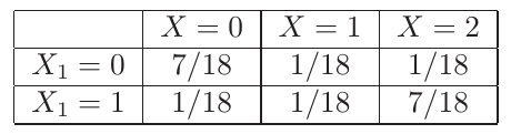
\strikeout off\uuline off\uwave off
x2 = 0
x2 = 1
\overset
x1 = 0
x2 = 1
x3 = 2
⎡⎢⎣
0.35431
0.072845
0.072845
0.072845
0.072845
0.35431
⎤⎥⎦
y|x1x2
y0
y1
y2
00
1
0
0
10
0
0.5
0.5
20
0
0.5
0.5
01
0.5
0.5
0
11
0.5
0.5
0
21
0
0
1
y|x1x2
y0
y1
y2
p(x1x2)
00
0.35431
0
0
0.35431
10
0
0.0364225
0.0364225
0.072845
20
0
0.0364225
0.0364225
0.072845
01
0.0364225
0.0364225
0
0.072845
11
0.0364225
0.0364225
0
0.072845
21
0
0
0.35431
0.35431
p(y)
0.427155
0.14569
0.427155
0.35431 + 2⋅0.0364225 = 0.427155
0.0364225⋅4 = 0.14569
N[7 ⁄ 18] = 0.388889
I(X1X2;Y) = H(Y) − H(Y|X1X2)
H(Y) = N⎡⎣2⋅0.427155⋅Log⎡⎣2, (1)/(0.427155)⎤⎦ + 0.14569⋅Log⎡⎣2, (1)/(0.14569)⎤⎦⎤⎦ = 1.45326
H(Y|X1X2 = 00) = H(Y|X1X2 = 21) = (1⋅log1) = 0
H(Y|X1X2 = 10) = p(Y = 1|(X1X2) = 10)log(p(Y = 1|(X1X2) = 10)) + p(Y = 1|(X1X2) = 10)log(p(Y = 1|(X1X2) = 10))
= (1)/(2)log22 + (1)/(2)log22 = 1
H(Y|X1X2 = 20) = H(Y|X1X2 = 01) = H(Y|X1X2 = 11) = log22 = 1
H(Y|X1X2) = ⎲⎳x1x2yp(x1x2)H(y|x1x2) = 2⋅0.35431⋅0 + 4⋅0.072845⋅1
4⋅0.072845⋅1 = 0.29138
I(X1X2;Y) = H(Y) − H(Y|X1X2) = 1.45326 − 0.29138 = 1.16188
Фала богу!!! Немам поим каде сум грешел до сега!
Барање на отпимална дистрибуција
——————————————————————————–——————————
y|x1x2
y0
y1
y2
00
1
0
0
10
0
0.5
0.5
20
0
0.5
0.5
01
0.5
0.5
0
11
0.5
0.5
0
21
0
0
1
y|x1x2
y0
y1
y2
p(x1x2)
00
a
0
0
a
10
0
0.5b
0.5b
b
20
0
0.5c
0.5c
c
01
0.5d
0.5d
0
d
11
0.5e
0.5e
0
e
21
0
0
f
f
p(y)
a + 0.5(d + e)
0.5(b + c + d + e)
f + 0.5(b + c)
\strikeout off\uuline off\uwave offH(Y|X1, X2) = ∑x1, x2p(x1, x2)⋅H(Y|X2 = x2, X1 = x1) = p(0, 0)H(Y|00) + p(10)H(Y|10) + p(20)H(Y|20) + p(01)H(Y|01) + p(11)H(Y|11) + p(2, 1)H(Y|21)
= p(00)⋅0 + \mathchoicep(10) + p(20) + p(01) + p(11)p(10) + p(20) + p(01) + p(11)p(10) + p(20) + p(01) + p(11)p(10) + p(20) + p(01) + p(11) + p(21)⋅0 го имав p(11) пропуштено!!!
p(Y = 0) = \mathchoicep(00) + (p(01) + p(11))/(2);p(00) + (p(01) + p(11))/(2);p(00) + (p(01) + p(11))/(2);p(00) + (p(01) + p(11))/(2); = a + (d + e)/(2)
p(Y = 1) = \mathchoice(p(10) + p(20))/(2) + (p(01) + p(11))/(2)(p(10) + p(20))/(2) + (p(01) + p(11))/(2)(p(10) + p(20))/(2) + (p(01) + p(11))/(2)(p(10) + p(20))/(2) + (p(01) + p(11))/(2) = (b + c)/(2) + (d + e)/(2); p(Y = 2) = \mathchoice(p(10) + p(20))/(2) + p(21)(p(10) + p(20))/(2) + p(21)(p(10) + p(20))/(2) + p(21)(p(10) + p(20))/(2) + p(21) = (b + c)/(2) + f
H(Y) = − ⎛⎝p(00) + (p(01) + p(11))/(2)⎞⎠⋅log2⎛⎝p(00) + (p(01) + p(11))/(2)⎞⎠ − ⎛⎝(p(10) + p(20))/(2) + (p(01) + p(11))/(2)⎞⎠⋅log2⎛⎝(p(10) + p(20))/(2) + (p(01) + p(11))/(2)⎞⎠ − ⎛⎝(p(10) + p(20))/(2) + p(21)⎞⎠⋅log2⎛⎝(p(10) + p(20))/(2) + p(21)⎞⎠
p(00) + p(10) + p(20) + p(01) + p(11) + p(21) = 1 p(00) = 1 − p(10) + p(20) + p(01) + p(11) + p(21)
\strikeout off\uuline off\uwave off\mathchoicep(00) = a; p(10) = b; p(20) = c; p(01) = d; p(11) = e; p(21) = f;p(00) = a; p(10) = b; p(20) = c; p(01) = d; p(11) = e; p(21) = f;p(00) = a; p(10) = b; p(20) = c; p(01) = d; p(11) = e; p(21) = f;p(00) = a; p(10) = b; p(20) = c; p(01) = d; p(11) = e; p(21) = f;
\strikeout off\uuline off\uwave offa + b + c + d + e + f = 1
\strikeout off\uuline off\uwave offH(Y) = − ⎛⎝a + (d + e)/(2)⎞⎠⋅log2⎛⎝a + (d + e)/(2)⎞⎠ − ⎛⎝(b + c)/(2) + (d + e)/(2)⎞⎠⋅log2⎛⎝(b + c)/(2) + (d + e)/(2)⎞⎠ − ⎛⎝(b + c)/(2) + f⎞⎠⋅log2⎛⎝(b + c)/(2) + f⎞⎠
\mathchoiceI(X1, X2;Y) = H(Y) − H(Y|X1X2) = − ⎛⎝a + (d + e)/(2)⎞⎠⋅log2⎛⎝a + (d + e)/(2)⎞⎠ − ⎛⎝(b + c)/(2) + (d + e)/(2)⎞⎠⋅log2⎛⎝(b + c)/(2) + (d + e)/(2)⎞⎠ − ⎛⎝(b + c)/(2) + f⎞⎠⋅log2⎛⎝(b + c)/(2) + f⎞⎠ − b − c − d − eI(X1, X2;Y) = H(Y) − H(Y|X1X2) = − ⎛⎝a + (d + e)/(2)⎞⎠⋅log2⎛⎝a + (d + e)/(2)⎞⎠ − ⎛⎝(b + c)/(2) + (d + e)/(2)⎞⎠⋅log2⎛⎝(b + c)/(2) + (d + e)/(2)⎞⎠ − ⎛⎝(b + c)/(2) + f⎞⎠⋅log2⎛⎝(b + c)/(2) + f⎞⎠ − b − c − d − eI(X1, X2;Y) = H(Y) − H(Y|X1X2) = − ⎛⎝a + (d + e)/(2)⎞⎠⋅log2⎛⎝a + (d + e)/(2)⎞⎠ − ⎛⎝(b + c)/(2) + (d + e)/(2)⎞⎠⋅log2⎛⎝(b + c)/(2) + (d + e)/(2)⎞⎠ − ⎛⎝(b + c)/(2) + f⎞⎠⋅log2⎛⎝(b + c)/(2) + f⎞⎠ − b − c − d − eI(X1, X2;Y) = H(Y) − H(Y|X1X2) = − ⎛⎝a + (d + e)/(2)⎞⎠⋅log2⎛⎝a + (d + e)/(2)⎞⎠ − ⎛⎝(b + c)/(2) + (d + e)/(2)⎞⎠⋅log2⎛⎝(b + c)/(2) + (d + e)/(2)⎞⎠ − ⎛⎝(b + c)/(2) + f⎞⎠⋅log2⎛⎝(b + c)/(2) + f⎞⎠ − b − c − d − e
Да симплифицирам:
y|x1x2
y0
y1
y2
00
1
0
0
10
0
0.5
0.5
20
0
0.5
0.5
01
0.5
0.5
0
11
0.5
0.5
0
21
0
0
1
y|x1x2
y0
y1
y2
p(x1x2)
00
a
0
0
a
10
0
0.5b
0.5b
b
20
0
0.5b
0.5b
b
01
0.5b
0.5b
0
b
11
0.5b
0.5b
0
b
21
0
0
a
a
p(y)
a + b
2b
a + b
I(X1, X2;Y) = H(Y) − H(Y|X1X2) = − 2(a + b)⋅log2(a + b) − (2b)⋅log2(2b) − 4b
2a + 4b = 1 → a = (1 − 4⋅b)/(2)
− 2⎛⎝(1 − 4⋅b)/(2) + b⎞⎠⋅log2⎛⎝(1 − 4⋅b)/(2) + b⎞⎠ − (2b)⋅log2(2b) − 4b = − 2⎛⎝(1 − 4⋅b + 2b)/(2)⎞⎠⋅log2⎛⎝(1 − 4⋅b + 2b)/(2)⎞⎠ − (2b)⋅log2(2b) − 4b = − 2⎛⎝(1 − 2⋅b)/(2)⎞⎠⋅log2⎛⎝(1 − 2⋅b)/(2)⎞⎠ − (2b)⋅log2(2b) − 4b
I(X1, X2;Y) = − (1 − 2⋅b)⋅log2⎛⎝(1 − 2⋅b)/(2)⎞⎠ − (2b)⋅log2(2b) − 4b
Од Maple добив:
(d)/(dp)(I(X1X2;Y)) = 0 → b = (1)/(8) ; a = (1 − 4⋅1 ⁄ 18)/(2) = (7)/(18)
maxpI(X1X2;Y) = \mathchoice1.16991.16991.16991.1699 bits
y|x1x2
y0
y1
y2
p(x1x2)
00
7 ⁄ 18
0
0
7 ⁄ 18
10
0
1 ⁄ 36
1 ⁄ 36
1 ⁄ 18
20
0
1 ⁄ 36
1 ⁄ 36
1 ⁄ 18
01
1 ⁄ 36
1 ⁄ 36
0
1 ⁄ 18
11
1 ⁄ 36
1 ⁄ 36
0
1 ⁄ 18
21
0
0
7 ⁄ 18
7 ⁄ 18
p(y)
4 ⁄ 9
1 ⁄ 9
4 ⁄ 9
Да ова е решението што го дава Cover за RUG = maxp(x1x2)I(X1X2;Y) докажано!!!
Пресметка на вториот член од cutset theorem.
p(y|x1x2) p(x1x2y)
y|x1x2
y0
y1
y2
00
1
0
0
10
0
0.5
0.5
20
0
0.5
0.5
01
0.5
0.5
0
11
0.5
0.5
0
21
0
0
1
y|x1x2
y0
y1
y2
p(x1x2)
p(x2)
00
7 ⁄ 18
0
0
7 ⁄ 18
x
10
0
1 ⁄ 36
1 ⁄ 36
1 ⁄ 18
y
20
0
1 ⁄ 36
1 ⁄ 36
1 ⁄ 18
y
01
1 ⁄ 36
1 ⁄ 36
0
1 ⁄ 18
y
11
1 ⁄ 36
1 ⁄ 36
0
1 ⁄ 18
y
21
0
0
7 ⁄ 18
7 ⁄ 18
x
p(y)
4 ⁄ 9
1 ⁄ 9
4 ⁄ 9
(p(x1x2))/(p(x2)) = p(x1|x2)
2x + 4y = 1 → x = (1 − 4y)/(2) → y = (1 − 2x)/(4)
I(X1;Y1|X2) = H(Y1|X2) − \cancelto0H(Y1|X1X2) = H(X1|X2) − \cancelto0H(X1|Y1X2) = H(Y1|X2) = H(X1|X2)?
H(X1|X2) = − ∑x1x2p(x1x2)logp(x1|x2) = − (4)/(18)log(1)/(18y) − (14)/(18)log⎛⎝(7)/(18x)⎞⎠ = (4)/(18)log18y + (14)/(18)log⎛⎝(18x)/(7)⎞⎠ = (4)/(18)log18⋅(1 − 2x)/(4) + (14)/(18)log⎛⎝(18x)/(7)⎞⎠
(d)/(dp)(I(X2;Y1|X2)) = 0 → x = 0.3181181 ;
(1 − 2⋅0.3181182)/(4) = 0.0909409
2⋅0.318181 + 4⋅0.0909409 = 1.00013
I(X2;Y1|X2) = 0.0453
——————————————————————————–——————————————————–
y|x1x2
y0
y1
y2
p(x1x2)
p(x2)
00
7 ⁄ 18
0
0
7 ⁄ 18
x
10
0
1 ⁄ 36
1 ⁄ 36
1 ⁄ 18
x
20
0
1 ⁄ 36
1 ⁄ 36
1 ⁄ 18
x
01
1 ⁄ 36
1 ⁄ 36
0
1 ⁄ 18
y
11
1 ⁄ 36
1 ⁄ 36
0
1 ⁄ 18
y
21
0
0
7 ⁄ 18
7 ⁄ 18
y
p(y)
4 ⁄ 9
1 ⁄ 9
4 ⁄ 9
x + y = 1 → y = 1 − x
H(X1|X2) = − ∑x1x2p(x1x2)logp(x1|x2) = − (2)/(18)log(1)/(18x) − (7)/(18)log⎛⎝(7)/(18x)⎞⎠ − (2)/(18)log(1)/(18y) − (7)/(18)log⎛⎝(7)/(18y)⎞⎠ = (2)/(18)log18x + (7)/(18)log⎛⎝(18x)/(7)⎞⎠ + (2)/(18)log18y + (7)/(18)log⎛⎝(18y)/(7)⎞⎠
= (2)/(18)log(182xy) + (7)/(18)log⎛⎝(182xy)/(72)⎞⎠ = (2)/(18)log(182x⋅(1 − x)) + (7)/(18)log⎛⎝(182)/(72)x⋅(1 − x)⎞⎠ = (2)/(18)log(324⋅(x − x2)) + (7)/(18)log⎛⎝(324)/(49)⋅(x − x2)⎞⎠
(182)/(72) = (324)/(49)
Со користење на Maple и изводи:
H(X1|X2) = 0.986
Нема потреба од изводи зошто се е дефинирано:
p(x1x2) p(x1|x2)
x1|x2
0
1
p(x1)
0
7 ⁄ 18
1 ⁄ 18
8 ⁄ 18
1
1 ⁄ 18
1 ⁄ 18
2 ⁄ 18
2
1 ⁄ 18
7 ⁄ 18
8 ⁄ 18
p(x2)
1 ⁄ 2
1 ⁄ 2
x1|x2
0
1
0
14 ⁄ 18
2 ⁄ 18
1
2 ⁄ 18
2 ⁄ 18
2
2 ⁄ 18
14 ⁄ 18
H(X1|X2) = (14)/(18)log2⎛⎝(18)/(14)⎞⎠ + (4)/(18)log2⎛⎝(18)/(2)⎞⎠
N⎡⎣(14)/(18)⋅Log⎡⎣2, (18)/(14)⎤⎦ + (4)/(18)⋅Log⎡⎣2, (18)/(2)⎤⎦⎤⎦ = 0.986427
Веројатно треба со башка вредности за p(x1x2):
p(x1x2) p(x1|x2)
x1|x2
0
1
p(x1)
0
a
b
a + b
1
b
b
2b
2
b
a
a + b
p(x2)
a + 2b
a + 2b
p(x2)
1 ⁄ 2
1 ⁄ 2
x1|x2
0
1
0
2a
2b
1
2b
2b
2
2b
2a
2a + 4b = 1 → b = (1 − 2a)/(4) → a + 2b = (1)/(2)
H(X1|X2) = − ∑x1x2p(x1x2)logp(x1|x2) = 2⋅a⋅log(1)/(2a) + 4⋅b⋅log(1)/(2b) = 2⋅a⋅log(1)/(2a) + 4⋅(1 − 2a)/(4)⋅log(4)/(2 − 4a)
Maple
a = 1 ⁄ 6
b = (1 − 2⋅1 ⁄ 6)/(4) = (1)/(6)
I(X1;Y1|X2) = H(X1|X2) = 1.585
Уште еднаш пресметка на вториот член од Cutset Theorem
y|x1x2
y0
y1
y2
00
1
0
0
10
0
0.5
0.5
20
0
0.5
0.5
01
0.5
0.5
0
11
0.5
0.5
0
21
0
0
1
y|x1x2
y0
y1
y2
p(x1x2)
00
a
0
0
a
10
0
0.5b
0.5b
b
20
0
0.5b
0.5b
b
01
0.5b
0.5b
0
b
11
0.5b
0.5b
0
b
21
0
0
a
a
p(y)
a + b
2b
a + b
I(X1, X2;Y) = H(Y) − H(Y|X1X2) = − 2(a + b)⋅log2(a + b) − (2b)⋅log2(2b) − 4b
2a + 4b = 1 → a = (1 − 4⋅b)/(2)
− 2⎛⎝(1 − 4⋅b)/(2) + b⎞⎠⋅log2⎛⎝(1 − 4⋅b)/(2) + b⎞⎠ − (2b)⋅log2(2b) − 4b = − 2⎛⎝(1 − 4⋅b + 2b)/(2)⎞⎠⋅log2⎛⎝(1 − 4⋅b + 2b)/(2)⎞⎠ − (2b)⋅log2(2b) − 4b = − 2⎛⎝(1 − 2⋅b)/(2)⎞⎠⋅log2⎛⎝(1 − 2⋅b)/(2)⎞⎠ − (2b)⋅log2(2b) − 4b
I(X1, X2;Y) = − (1 − 2⋅b)⋅log2⎛⎝(1 − 2⋅b)/(2)⎞⎠ − (2b)⋅log2(2b) − 4b
Од Maple добив:
(d)/(db)(I(X1X2;Y)) = 0 → b = (1)/(1g(8) ; a = (1 − 4⋅1 ⁄ 18)/(2) = (7)/(18)
maxpI(X1X2;Y) = \mathchoice1.16991.16991.16991.1699 bits
y|x1x2
y0
y1
y2
p(x1x2)
00
7 ⁄ 18
0
0
7 ⁄ 18
10
0
1 ⁄ 36
1 ⁄ 36
1 ⁄ 18
20
0
1 ⁄ 36
1 ⁄ 36
1 ⁄ 18
01
1 ⁄ 36
1 ⁄ 36
0
1 ⁄ 18
11
1 ⁄ 36
1 ⁄ 36
0
1 ⁄ 18
21
0
0
7 ⁄ 18
7 ⁄ 18
p(y)
4 ⁄ 9
1 ⁄ 9
4 ⁄ 9
Да ова е решението што го дава Cover за RUG = maxp(x1x2)I(X1X2;Y) докажано!!!
За време на читање на докторатот
I(X1;Y1|X2) = H(Y1|X2) − H(Y1|X1X2) = H(Y1) = H(X1) = − p1log(p1) − p2log(p2) − p3log(p3) = − 2⋅(a + b)log(a + b) − 2b⋅log(2b)
p(x1x2)
x1 ⁄ x2
0
1
p(x1)
0
a
b
a + b
1
b
b
2b
2
b
a
a + b
p(x2)
a + 2b
a + 2b
− 2⋅(a + b)log(a + b) − 2b⋅log(2b) = − (1 − 2⋅b)⋅log2⎛⎝(1 − 2⋅b)/(2)⎞⎠ − (2b)⋅log2(2b) − 4b
a = (1 − 4⋅b)/(2)
− 2⋅((1 − 4⋅b)/(2) + b)log⎛⎝(1 − 4⋅b)/(2) + b⎞⎠ − 2b⋅log(2b) = − (1 − 2⋅b)⋅log2⎛⎝(1 − 2⋅b)/(2)⎞⎠ − (2b)⋅log2(2b) − 4b
(1 − 4⋅b)/(2) + b = (1 − 4⋅b + 2b)/(2) = (1 − 2⋅b)/(2)
− 2⋅((1 − 2⋅b)/(2))log⎛⎝(1 − 2⋅b)/(2)⎞⎠ − 2b⋅log(2b) = − (1 − 2⋅b)⋅log2⎛⎝(1 − 2⋅b)/(2)⎞⎠ − (2b)⋅log2(2b) − 4b → b = 0
Значи двете функции се сечат за b = 0.
(d)/(db)I(X1;Y1|X2) = 0 → b = (1)/(6) → a = (1)/(6) → I(X1;Y1|X2) = 1.585
Дефинитивно I(X1X2;Y) ≥ I(X1;Y1|X2)
Пак истото се добива.
Последно што пробав во Maple да барам извод по a после по b и да ги решам равенките после. Не се добиваат добри резултати.
2 Achievability of C in Theorems 1,2,3
The achievability of
\mathchoiceC0 = supp(x1)maxx2I(X1;Y|x2)C0 = supp(x1)maxx2I(X1;Y|x2)C0 = supp(x1)maxx2I(X1;Y|x2)C0 = supp(x1)maxx2I(X1;Y|x2) in Theorem 2 follows immediately form Shannon’s basic result
[5] if we set
X2i = x2, i = 1, 2, ... . Also the achievability of
CFB in Theorem 3 is a simple corollary of Theorem 1,
when it is realized that the feedback relay channel is a degraded relay channel. The converses will be delayed until Section III.
We are left only with the proof of Theorem 1 - the achievability of C for the degraded relay channel. We begin with a brief outline of the proof. We consider B blocks , each of n symbols. A sequence of B − 1 messages wi ∈ [1, 2nR], i = 1, 2, ..., B − 1 will be sent over the channel in nB transmissions. (Note that as B → ∞, for fixed n, the rate \mathchoiceR(B − 1) ⁄ BR(B − 1) ⁄ BR(B − 1) ⁄ BR(B − 1) ⁄ B is arbitrary close to R.)
Многу е важно да се сконта дека праќа B − 1 пораки во B блокови. Ако претпоставиш дека еден блок се прaќа во една употреба на каналот (на пример n паралелни бинарни канали=еден блок) тогаш доколку нема грешки во преносот во приемникот ќе препознаеш B-1 блокови за B употреби на каналот т.е капацитетот ќе биде (B − 1) ⁄ B. Секогаш потсеќај се на noisy typewriter. Што и да правиш тој пола од буквите ги греши (шум) па на излез препознаваш само 13 од вкупно 26. Затоа капацитетот во бити беше log2(13) или во букви 0.5. (после EIT) Мислам дека едната порака не е стигната во приемникот затоа што сеуште се процесира во релето.
In each n-block b = 1, 2, ..., B we shall use the same doubly indexed set of codewords
We shall also need a partition
The partition S will allow us to send information to the receiver using the random binning proof of the source coding theorem of Seplian and Wolf [7].
The choice of C and S achieving C will be random, but the description of the random code and partition will be delayed until the use of the code is described. For the time being, the code should be assumed fixed.
We pick up the story in block i − 1. First, let us assume that the receiver y knows wi − 2 and si − 1 at the end of block i − 1. Let us also assume that the relay receiver knows wi − 1. We shall show that a good choice of {C, S} will allow the receiver to know (wi − 1, si) and the relay receiver to know wi at the end of block i (with probability of error ≤ ϵ). Thus the information state (wi − 1, si) of the receiver propagates forward, and a recursive calculation of the probability of error can be made, yielding probability of error ≤ Bϵ.
We summarize the use of the code as follows.
Transmission in block i − 1: x1(wi − 1|si − 1), x2(si − 1).
Received signals in block i − 1: Y1(i − 1), Y(i − 1) .
Computation at the end of block i − 1: the relay receiver
Y1(i − 1) is assumed to know
wi − 1.
The integer wi − 1 falls in some cell of the partition S. Call the index of this cell si. Then the relay is prepared to send
x2(si) in block
i. Transmitter
x1 also computes
si from
wi − 1.
Thus si will furnish the basis for cooperative resolution of the y uncertainty about wi − 1.
Remark: In the first block, the relay has no information s1 necessary for cooperation. However any good sequence x2 will allow the block Markov scheme to get started, and the slight loss in rate in the first block becomes asymptotically negligible as the number of blocks B → ∞.
Transmission in block i: x1(wi|si), x2(si).
Received signals in block i: y1(i), y(i).
Computation at end of block i: 1) The relay calculates wi from y1(i). 2) The unique jointly typical x2(si) with the received y(i) is calculated. Thus the si is known to the receiver. 3) The receiver calculates his ambiguity set J(\mathnormaly(i − 1)) i.e., the set of all wi − 1 such that (x1(wi − 1|si − 1), x2(si − 1), y(i − 1)) are jointly ϵ-typical.
The receiver then intersects \strikeout off\uuline off\uwave offJ(\mathnormaly(i − 1)) and the cell Ssi. By controlling the size of J, we shall (1 − ϵ)-guarantee that this intersection has one and only one member- the correct value wi − 1. We conclude that the receiver y(i) has correctly computed (wi − 1, si) from (wi − 2, si − 1)
\strikeout off\uuline off\uwave offЗошто му треба (wi − 2, si − 1)???
and (y(i − 1), y(i)).
Proof of achievability of C in Theorem 1:
We shall use the code as outlined previously in this section. It is important to note that, although Theorem 1 treats degraded relay channels, the proof of achievability of C and all constructions in this section apply without change to arbitrary relay channels. It is only in the converse that degradedness is needed to establish that the achievable rate C is indeed the capacity. the converse is proved in Section III.
We shall now describe the random codes. Fix a probability mass function p(x1, x2).
First generate at random M0 = 2nR0 independent identically distributed n-sequences in X\mathnormaln\mathnormal2 , each drawn according to p(x2) = ∏ni = 1p(x2i). Index them as x2(s), s ∈ [1, 2nR0]. For each x2(s),
Ова е многу важно! Сака да каже дека за секоj bin s генерираш посебна кодна подкнига од 2nR елементи. Вкупната кодна книга содржи 2nR0 x2nR1 елементи.
generate M = 2nR conditionally independent n-sequences x1(w|s), w ∈ [1, 2nR] drawn according to p(x1|x2(s)) = ∏ni = 1p(x1i|x2i(s)). This defines a random code book C\mathnormal = {x1(w|s), x2}.
Reveal the assignments to both the encoder and the decoder.
Тhe random partition S\mathnormal = {S1, S2..., S2nR0} of {1, 2, ..., 2nR} is defined as follows. Let each integer w ∈ [1, 2nR] be assigned independently, according to a uniform distribution over the indices s = 1, 2, ..., 2nR0, to cell Ss. We shall use the functional notation s(w) to denote the index of the cell in which w lies.
Reveal the s(w) assignments to Relay and Destination.
We recall some basic results concerning typical sequences. Let
{X(1), X(2)..., X(k)} denote a finite collection of discrete random variables with some fixed joint distribution
p(x(1), x(2), ..., x(k)), for
(x(1), x(2), ..., x(k)) ∈ X(1) xX(2) x...xX\mathnormal(k).
Let S denote an ordered subset of these random variables, and consider n independent copies of S. Thus
Let \mathchoiceN(s;s)N(s;s)N(s;s)N(s;s) be the number of indices i ∈ {1, 2, ..., n} such that Si = s. By the law of large numbers, for any subset S of random variables and for all s ∈ S,
N(s;s) го замислувам во експеримент на фрлање на коцка како број на пати коцката паѓа на одредена бројка. n го замислувам е колку пати е направен експериментот (фрлање на коцка). За подолу истото го замислуваш за случаен процес кој се состои од секвенца од k коцки.
18.06.14
Внимавај не се работи за секвенца од случајни променливи како гореш што замислувам туку се работи за секвенца од случајни процеси.
Последното замислување е следново. Множеството s е секвенца од секвенци од кое вадиш примерок од n обзервации. (1)/(n)N(s, s) сака да каже дека
количникот од бројот на појавувања на секвенцата s во примерокот од обзервации и вкупната должина на примерокот, стреми кон веројатноста на појавување на секвенцата s.
Also
Convergence in
20↑ and
21↑ takes place simultaneously with probability one for all
2k subsets
S ⊆ {X(1), X(2), ..., X(k)}
Consider the following definition of joint typicality.
The set Aϵ of ϵ-typical n-sequences (x(1), x(2), ..., x(k)) is defined by:
Aϵ(X(1), X(2)..., X(k)) = Aϵ = ⎧⎩(x(1), x(2), ..., x(k)):||(1)/(n)N(x(1), x(2), ..., x(k);x(1), x(2), ..., x(k)) − p(x(1), x(2), ..., x(k))|| <
< ϵ||X(1) xX(2) x...xX\mathnormal(k)|| for (x(1), x(2), ..., x(k)) ∈ X(1) xX(2) x...xX\mathnormal(k)}
where ||ℛ|| is cardinality of the set ℛ.
Remark: The definition of typicality, sometimes called strong typicality
Се потсетив на дефиницијата на strong typicality во EIT Chapter 15.8.
can be found in work of Wolfowitz
[13] and Berger
[12]. Strong typicality implies (week) typicality used in
[8],
[14]. The distinction is not needed until the proof of Theorem 6 in Section VI of this paper.
The following is a version of the asymptotic equipartition property involving simultaneous constraints [12],
[14].
For any ϵ > 0 , there exist and integer n such that Aϵ(S) satisfies
i) Pr{Aϵ(S)} ≥ 1 − ϵ, for all S ⊆ {X(1), X(2)..., X(k)}
ii) s ∈ Aϵ(S) ⇒ || − (1)/(n)logp(s) − H(s)|| ≤ ϵ
We shall need to know the probability that conditionally independent sequences are jointly typical. Let S1, S2 and S3 be three subsets of X(1), X(2)..., X(k). Let S’1, S’2 be conditionally independent given S3 with the marginals
p(s1|s3) = ∑s2p(s1, s2, s3) ⁄ p(s3)
p(s2|s3) = ∑s1p(s1, s2, s3) ⁄ p(s3)
∑s2(p(s1, s2, s3))/(p(s3)) = ∑s2p(s1, s2, s3|s3) = ∑s2p(s1, s3|s3)⋅p(s2, s3|s3) = p(s1, s3|s3)∑s2p(s2, s3|s3) = p(s1, s3)⋅1;
The following lemma is provided in
[14].
Let (S1, S2, S3) ~ ∏ni = 1p(s1i, s2i, s3i) and \strikeout off\uuline off\uwave off(S’1, S’2, S’3) ~ ∏ni = 1p(s1i|s3i)p(s2i|s3i)p(s3i). Then, for n such that P{Aϵ(S1, S2, S3)} > 1 − ϵ,
(1 − ϵ)2 − n⋅(I(S1;S2|S3 + 7⋅ϵ) ≤ P{(S’1, S’2, S3) ∈ Aϵ(S1, S2, S3)} ≤ 2 − n⋅(I(S1;S2|S3) − 7ϵ)
Ова лема мислам ја дава веројатноста некоја друга секвенца да припаѓа на типичното множество. (потсeти се на EIT Theorem 7.6.1 - Joint AEP)
18.06.2014
Да ова е всушност Теоремата 15.2.3 од EIT
Доказот од EIT е:
P{(S1’, S2’, S3’) ∈ A(n)ϵ} = ⎲⎳(s1, s2, s3) ∈ A(n)ϵp(s3)p(s1|s3)p(s2|s3)≐|A(n)ϵ(S1S2S3)|2 − n(H(S3)±2ϵ)2 − n(H(S1|S3)±2ϵ)2 − n(H(S2|S3)±2ϵ)
≐2n(H(S1S2S3)±ϵ) − n(H(S3)±ϵ) − n(H(S1|S3)±2ϵ) − n(H(S2|S3)±2ϵ)≐2 − n(I(S1;S2|S3)±6ϵ)
n(H(S1S2S3)±ϵ) − n(H(S3)±ϵ) − n(H(S1|S3)±2ϵ) − n(H(S2|S3)±2ϵ) =
n[H(S1S2S3)±ϵ − H(S3)∓ϵ − H(S1|S3)∓2ϵ − H(S2|S3)∓2ϵ]
n[H(S1S2S3) − H(S3) − H(S1|S3) − H(S2|S3)] = (*)
I(S1;S2|S3) = H(S1|S3) − H(S1|S2S3)
H(S1S2S3) = H(S3) + H(S2|S3) + H(S1|S2S3)
(*) = n[\cancelH(S3) + \cancelH(S2|S3) + H(S1|S2S3) − \cancelH(S3) − H(S1|S3) − \cancelH(S2|S3)] = − n⋅I(S1;S2|S3)
Ако се земат во предвид проментие на знаците во
± тогаш:
n[H(S1S2S3)±ϵ − H(S3)∓ϵ − H(S1|S3)∓2ϵ − H(S2|S3)∓2ϵ] = − n⋅(I(S1;S2|S3)±4ϵ)
Ако не се земат во предвид промените на знаците во
± тогаш:
n[H(S1S2S3)±ϵ − H(S3)±ϵ − H(S1|S3)±2ϵ − H(S2|S3)±2ϵ] = − n⋅(I(S1;S2|S3)±6ϵ)
Повторување од EIT
recall AEP from EIT textbook let: X = Xn1, Y = Yn1
2 − n(H(X, Y) + ϵ) ≤ p(X, Y) ≤ 2 − n(H(X, Y) − ϵ)
1) Pr(p(X, Y) ∈ A(n)ϵ) ≥ 1 − ϵ
2) (1 − ϵ)⋅2n(H(X, Y) − ϵ) ≤ |A(n)ϵ| ≤ 2n(H(X, Y) + ϵ)
3) (1 − ϵ)2 − n(I(X, Y) + 3ϵ) ≤ Pr((\widetildeX, \widetildeY) ∈ A(n)ϵ) ≤ 2 − n(I(X, Y) − 3ϵ)
1 = ⎲⎳x, yp(X, Y) ≥ ⎲⎳x, y2 − n(H(X, Y) + ϵ) ≥ ⎲⎳(x, y) ∈ A(n)ϵ2 − n(H(X, Y) + ϵ) = |A(n)ϵ|⋅2 − n(H(X, Y) + ϵ) ⇒ |A(n)ϵ| ≤ 2n(H(X, Y) + ϵ)
1 − ϵ ≤ ⎲⎳(X, Y) ∈ A(n)ϵp(X, Y) ≤ ⎲⎳(X, Y) ∈ A(n)ϵ2 − n(H(X, Y) − ϵ) = |A(n)ϵ|⋅2 − n(H(X, Y) − ϵ) ⇒ |A(n)ϵ| ≥ (1 − ϵ)⋅2n(H(X, Y) − ϵ)
\strikeout off\uuline off\uwave off
Pr((\widetildeX, \widetildeY) ∈ A(n)ϵ) = ⎲⎳(\widetildeX, \widetildeY) ∈ A(n)ϵp(\widetildeX, \widetildeY) = |A(n)ϵ|p(\widetildeX)⋅p(\widetildeY) ≤ 2n(H(X, Y) + ϵ)⋅2 − n(H(\widetildeX) − ϵ)⋅2 − n(H(\widetildeY) − ϵ) = 2n⋅H(X, Y) + nϵ − nH(\widetildeX) + nϵ − nH(\widetildeY) + nϵ
= 2 − n⋅( − H(X, Y) + H(\widetildeX) + H(\widetildeY)) + 3nϵ = 2 − n⋅( − H(\widetildeY|\widetildeX) + H(\widetildeY)) + 3nϵ = 2 − n(I(\widetildeX:\widetildeY) − 3ϵ) ⇒ Pr((\widetildeX, \widetildeY) ∈ A(n)ϵ) ≤ 2 − n(I(\widetildeX;\widetildeY) − 3ϵ)
Pr((\widetildeX, \widetildeY) ∈ A(n)ϵ) = ⎲⎳(\widetildeX, \widetildeY) ∈ A(n)ϵp(\widetildeX, \widetildeY) = ⎲⎳(\widetildeX, \widetildeY) ∈ A(n)ϵp(\widetildeX)⋅p(\widetildeY) = |A(n)ϵ|p(\widetildeX)⋅p(\widetildeY) ≥ (1 − ϵ)⋅2n(H(X, Y) − ϵ)⋅2 − n(H(\widetildeX) + ϵ)⋅2 − n(H(\widetildeY) + ϵ) =
(1 − ϵ)⋅2nH(X, Y) − n⋅ϵ − nH(\widetildeX) − n⋅ϵ − nH(\widetildeY) − n⋅ϵ = (1 − ϵ)⋅2 − n( − H(X, Y) + H(\widetildeX) + H(\widetildeY)) − 3n⋅ϵ = (1 − ϵ)⋅2 − n( − H(\widetildeY|\widetildeX) + H(\widetildeY)) − 3n⋅ϵ = (1 − ϵ)⋅2 − n(I(X;Y) + 3⋅ϵ)
⇒ Pr((\widetildeX, \widetildeY) ∈ A(n)ϵ) ≥ (1 − ϵ)⋅2 − n(I(X;Y) + 3⋅ϵ) i.e. (1 − ϵ)⋅2 − n(I(X;Y) + 3⋅ϵ) ≤ Pr((\widetildeX, \widetildeY) ∈ A(n)ϵ) ≤ 2 − n(I(\widetildeX;\widetildeY) − 3ϵ)
Let wi ∈ [1, 2nR] be the next index to be sent in block i, and assume that wi − 1 ∈ Ssi. The encoder then sends x1(wi|si). The relay has an estimate
ŵ̂i − 1 of the previous index
wi − 1 ∈ Ssi. (This will be made precise in the decoding section.)
Assume that ŵ̂i − 1 ∈ Sŝ̂i. Then the relay encoder sends the codeword x2(sî̂) in block i.
Ова е многу важно! Значи релето гледа во којa клетка припаѓа примениот сигнал и врз основ на индексот на таа клетка го праќа содветниот симбол x2 во наредниот блок.
i
1
2
3
4
...
i
...
b
X1
x1(w1|s1)
x1(w2|s2)
x1(w3|s3)
x1(w4|s4)
x1(wj|sj)
x1(wb|sb)
X2
0
x2(s2)
x2(s3)
x2(s4)
x2(sj)
x2(sb)
Y
y(1)
y(2)
y(3)
y(4)
y(j)
y(b)
We assume that at the end of block (i − 1) the receiver knows (w1, w2, ...wi − 2) and (s1, s2, ..., si − 1) and the relay knows (w1, w2, ...wi − 1) and consequently \mathchoice(s1, s2, ..., si)(s1, s2, ..., si)(s1, s2, ..., si)(s1, s2, ..., si).
The decoding procedures at the end of block i are as follows.
\mathchoice1.1.1.1. Knowing si, and upon receiving y1(i), the relay receiver estimates the message of the transmitter wî̂ = w if there exists a unique w such that (x1(w|si), x2(si), y1(i)) are jointly ϵ-typical. Using Lemma 2, it can be shown that \mathchoicewî̂ = wiwî̂ = wiwî̂ = wiwî̂ = wi with arbitrary small probability of error if
and n is sufficiently large.
Овој израз ја дефинира горната граница на брзината на пренос во каналот!!! Односно изразот R < I(X1, X2;Y).
\mathchoice2.2.2.2. The
receiver declares that
sî = s was sent if there exist one and only one
s such that
(x2(s), Y(i)) are jointly
ϵ -typical. From Lemma 2 we know that
si can be decoded with arbitrary small probability of error if
si can be decoded with arbitrarily small probability of error if si takes on less than 2nI(X2;Y) values , i.e. if
and n is sufficiently large.
\mathchoice3.3.3.3. Assuming that si is decoded successfully at the receiver, then ŵi − 1 = w is declared to be the index sent in bloc i − 1 if there is a unique \mathchoicew ∈ Ssi∩ℒ\mathnormal(y(i − 1))w ∈ Ssi∩ℒ\mathnormal(y(i − 1))w ∈ Ssi∩ℒ\mathnormal(y(i − 1))w ∈ Ssi∩ℒ\mathnormal(y(i − 1)). It will be shown that if n is sufficiently large and if
then \mathchoiceŵi − 1 = wi − 1ŵi − 1 = wi − 1ŵi − 1 = wi − 1ŵi − 1 = wi − 1 with arbitrary small probability of error.
Претпоставувам дека ℒ(y(i-1)) функцијата за декодирање (decoding function - g(...)) која го дава излезниот симбол во приемникот. Да ама излезот од оваа функција е множество. Подолу има формула за кардиналност на тоа множество. Веројатно го дава множеството на можни излезни симболи.
25.06.2014
Накратко сакам да ја опишам целата постапка како функционира релејниот систем и како се остварува кооперацијата.
Имаш w ∈ [1, ..., 2nR] пораки односно Xn(w) кодни зборови кои сакаш да ги пренесеш. Прво ги складираш случајно во 2nR0 кошнички. Ако бројот на кошнички е доволно голем можеш да очекуваш во секоја кошничка да има само еден типичен коден збор. Со тоа ја формираш коднага книга x(w|s(w)). Кодната книга ја соопштуваш на релето и дестинацијата. Кога ќе го испратиш еден кодниот зборо x1(wi − 1|si) тој се декодира во релето и во дестинацијата. Релето е поблиску до изворот од дестинацијата и затоа неговата естимација на овој симбол е поточна (посигурна) од естимациајта во дестинацијата. Со други зборови на дестинацијата и е потребна дополнителна информација за да со поголема сигурност го реконструира испратениот коден збор. Таа дополнителна информација ќе ја добие во наредниот блок кога изворот ќе го испрати x1(wi|si + 1). Во меѓувреме релето го реконструирал wi − 1 (ŵ̂i − 1)од приемениот деградиран x1(wi − 1|s) т.е. од y1 (гледа во претходно дистрибуираната кодна книга), а дестинацијата врз основ на деградиранот x1(wi − 1|si) т.е y2 го идентивикува множеството на можни кодни зборови ℒ(y(i − 1)). Кога изворот ќе го прати x1(wi|si + 1) тогаш релето ќе го прати x2(si). Дестинацијата врз основ на x2(ŝ̂i) ќе го реконструира ŝi т.е. ќе ја естимира коншничката каде припаѓал wi − 1. Во кошничката може да припаѓаат повеќе кодни зборови. Пресекот меѓу кошничката и множеството на можни кодни зборови: Ssi∩ℒ(y(i − 1)) ќе ја дате точната естимација на испратената порака wi − 1.
Гледаш во i-от тајмслот приемникот го декодира wi − 1, a предаватеот всушност го пратил wi, Ова wi е наменето за релето за да тоа го најде si + 1 кое ќе го прати како x(si + 1) во наредниот тајмслот кога предавателот ќе испраќа x(wi + 1|si + 1) .
Заттоа вкупната информација е R ≈ I(X1;Y|X2) + R0 ја сумираш информацијата пратена од изворот до релето во претходниот слот и информацијата пратена од релето кон приемникот во сегашниот слот.
30.07.2014
Не е баш вака ова е сума од информацијата од изворот до релето и информацијата од изворот до дестинацијата.
Thus combining
24↑ and
25↑ yields
R < I(X1, X2;Y)
(R < I(X1;Y|X2) + R0 < I(X1;Y|X2) + I(X2;Y) = I(X1, X2;Y))
, the first term in the capacity expression in Theorem 1. The second term is given by constraint
23↑.
Calculation of Probability of Error:
For the above scheme, we will declare an error in block i if one or more of the following events occurs.
E0i (x1(wi|si), x2(si), y1(i), y(i)) is not jointly ϵ-typical.
E1i in decoding step 1, there exists w̃ ≠ wi such that x1((w̃|si), x2(si), Y1(i)) is jointly typical.
Сака да каже дека не постои unique w.
E2i in decoding step 2, there exist s̃ ≠ si such that (x2(s̃), y(i)) is jointly typical.
Сака да каже дека постои и друго s = s̃ така што (x2(s̃), Y(i)) се jointly typical.
E3i decoding step 3 fails. Let E3i = E’3i∪E’’3i , where
E’3i wi − 1∉Ssi∩ℒ\mathnormal(y(i − 1))
Сака да каже дека не може да се најде такво w такаш што w ∈ Ssi∩ℒ\mathnormal(y(i − 1)).
E’’3i there exists w̃ ∈ [1, 2nR], w̃ ≠ wi − 1, such that w̃ ∈ Ssi∩ℒ\mathnormal(y(i − 1)).
Сака да каже дека постои и другo w = w̃ за кое што исто така важи w̃ ∈ Ssi∩ℒ\mathnormal(y(i − 1)) .
Now we bound the probability of error over the B n-blocks. Let \mathchoiceW = (W1, W2, .., WB − 1, ∅)W = (W1, W2, .., WB − 1, ∅)W = (W1, W2, .., WB − 1, ∅)W = (W1, W2, .., WB − 1, ∅) be the transmitted sequence of indices. We assume the indices Wi are independent identically distributed random variables uniformly distributed on [1, 2nR] . The relay estimates W to be \mathchoiceŴ̂ = (Ŵ̂1, Ŵ̂2, ...Ŵ̂B − 1, ∅)Ŵ̂ = (Ŵ̂1, Ŵ̂2, ...Ŵ̂B − 1, ∅)Ŵ̂ = (Ŵ̂1, Ŵ̂2, ...Ŵ̂B − 1, ∅)Ŵ̂ = (Ŵ̂1, Ŵ̂2, ...Ŵ̂B − 1, ∅). The receiver estimates \mathchoiceŜ = (∅, Ŝ2, Ŝ3, ...ŜB)Ŝ = (∅, Ŝ2, Ŝ3, ...ŜB)Ŝ = (∅, Ŝ2, Ŝ3, ...ŜB)Ŝ = (∅, Ŝ2, Ŝ3, ...ŜB) and \strikeout off\uuline off\uwave off\mathchoiceŴ = (∅, Ŵ1, Ŵ2, .., ŴB − 1)Ŵ = (∅, Ŵ1, Ŵ2, .., ŴB − 1)Ŵ = (∅, Ŵ1, Ŵ2, .., ŴB − 1)Ŵ = (∅, Ŵ1, Ŵ2, .., ŴB − 1). Define the error events Fi for \uuline default\uwave defaultdecoding errors in block i\strikeout off\uuline off\uwave off by:
19.06.14
Дури сега во суштина ја сконтав
26↑ и зошто само
Ŵ ≠ W\mathchoicei − 1i − 1i − 1i − 1. Види ги подвлекувањата во црвено. Тие всушност го потврдуваат она што го кажав во
13↑
Се ми се чини дека треба наместо Fi овде да биде Fi − 1. Не, не, не со Fci − 1 во наредните изрази сака да исклучи дека во претходниот блок се случила грешка.
\strikeout off\uuline off\uwave off
\strikeout off\uuline off\uwave offНе знам што значи индексот „c”. Претпоставив, а потоа и видов потврда на yahoo answers дека се работи за негација т.е. комплемент.
Да така е ов EIT Chapter 15 постојано ја користи таа нотација.
We have argued in encoding-decoding steps 1 and 2 that:
негација од дисјункција е конјукција од негациите (de morgan law).
Ова е логично негација од 26↑ согласно законот на de morgan вели дека \strikeout off\uuline off\uwave offŴ̂i − 1 = Wi − 1 and Ŵi − 1 = Wi − 2 and Ŝi − 1 = Si − 1 (негација од дисјункција е конјукција од поединечните негации.). Од друга страна тоа значи дека\uuline default\uwave default (x1(w|si), x2(si), y1(i)) се jointly ϵ-typical што е спротивно на E0i.
Зошто дели со 4B???
Сака да каже дека штом \strikeout off\uuline off\uwave offимаме настанEc0i\uuline default\uwave default кој вели дека не е точно дека \strikeout off\uuline off\uwave off(x1(wi|si), x2(si), y1(i), y(i)) не се типични од една страна и од друга страна настан (Fci − 1) кој вели дека се случило Ŵ̂i − 1 = Wi − 1 and Ŵi − 1 = Wi − 2 and Ŝi − 1 = Si − 1 тогаш веројатност да се случи настан (E1i) \uuline default\uwave defaultw̃ ≠ wi така што (x1(w̃|si), x2(si), Y1(i)) се здружено типични е многу мала. Слично е и толкувањето за 29↓.
Малку ме бунат сините (cyan) индексите ама и со нив е ОК толкувањето. E настаните се за сегашниот тајмслот, а F настаните за претхондиот.
We now show that \strikeout off\uuline off\uwave offP(E3i∩Ec2i∩Ec0i|Fci − 1) can be made small.
If
\mathchoiceR < I(X1;Y|X2) + R0 − 7ϵR < I(X1;Y|X2) + R0 − 7ϵR < I(X1;Y|X2) + R0 − 7ϵR < I(X1;Y|X2) + R0 − 7ϵ,
then for sufficiently large n
\mathchoiceProof:Proof:Proof:Proof:First we bound E{||L\mathnormal(Y(i − 1))|||\mathnormalFci − 1}, where ||ℒ|| denotes the number of elements in ℒ. Let
The cardinality of L\mathnormal(y(i − 1)) is the random variable
and
E{||ℒ\mathnormal(y(i − 1))|||\mathnormalFci − 1} = \mathchoiceE{ψ(wi − 1|y(i − 1))|Fci − 1}E{ψ(wi − 1|y(i − 1))|Fci − 1}E{ψ(wi − 1|y(i − 1))|Fci − 1}E{ψ(wi − 1|y(i − 1))|Fci − 1} + \mathchoice ⎲⎳w ≠ wi − 1E{ψ(w|y(i − 1))|Fci − 1} ⎲⎳w ≠ wi − 1E{ψ(w|y(i − 1))|Fci − 1} ⎲⎳w ≠ wi − 1E{ψ(w|y(i − 1))|Fci − 1} ⎲⎳w ≠ wi − 1E{ψ(w|y(i − 1))|Fci − 1}
From Lemma 2 we obtain, for each w ∈ [1, M],
(Веројатноста некоја друга секвенца да припаѓа на типилното множество е мала)
Therefore (by introducing
33↑ in
32↑)
E{||ℒ\mathnormal(y(i − 1))|||\mathnormalFci − 1} ≤ \cancelto зеленото од Eq341 + \cancelto портокаловото од Eq34(2nR − 1)⋅(2 − n(I(X1;Y|X2) − 7ϵ)) = 1 + 2nR⋅2 − n(I(X1;Y|X2) − 7ϵ) − 2 − n(I(X1;Y|X2) − 7ϵ) ≤ 1 + 2n⋅(R − I(X1;Y|X2) + 7ϵ)
The event Fci − 1 implies that wi − 1 ∈ L\mathnormal(y(i − 1)). Also Ec2i ⇒ ŝi = si ⇒ wi − 1 ∈ Ssi. Thus
E’3i вели дека се случил настанот \strikeout off\uuline off\uwave offwi − 1∉Ssi∩ℒ\mathnormal(y(i − 1)) што е во контрадикција со горното тврдење. Затоа веројатноста тој настан да се случи во вакви услови е 0.\uuline default\uwave default
Hence
P(E3i∩Ec2i∩Ec0i|Fci − 1) = P(E’’3i∩Ec2i∩Ec0i|Fci − 1) ≤ P{there exists w ≠ Wi − 1such that w ∈ ℒ\mathnormal(y(i − 1)∩Ssi|Fci − 1)} ≤
≤ E{ ⎲⎳\oversetw ≠ Wi − 1w ∈ ℒ\mathnormal(y(i − 1))P(w ∈ Ssi)|Fci − 1} ≤ E{||ℒ\mathnormal(y(i − 1))||⋅2 − nR0|Fci − 1} ≤ |\undersetВеројатностанекојадругасеквенцадаприпаѓанатипилнотомножествоемалаПретпоставувам дека P(w ∈ Ssi) = (1)/(2nR0)|
= 2 − nR0⋅E{||ℒ\mathnormal(y(i − 1))|||Fci − 1} ≤ | introduce Eq.35| ≤ 2 − nR0⋅{1 + 2n⋅(R − I(X1;Y|X2) + 7ϵ)}
Thus, if
\mathchoiceR0 > R − I(X1;Y|X2) + 7⋅ϵR0 > R − I(X1;Y|X2) + 7⋅ϵR0 > R − I(X1;Y|X2) + 7⋅ϵR0 > R − I(X1;Y|X2) + 7⋅ϵ then for sufficiently large n, P(E3i∩Ec2i∩Ec0i|Fci − 1) ≤ (ϵ)/(4B).
Proof of the lemma
But from
24↑ we required:
\mathchoiceR0 < I(X2;Y)R0 < I(X2;Y)R0 < I(X2;Y)R0 < I(X2;Y).
Combining the two constraints, R0 drops out, leaving
The probability of error is given by
Обичната унија ја разбирам. Имено вели грешка се случува или во блокот i = 1 или во i = 2 или ... или во i = B. Ова со одземањето под знакот на унијата не го контам!? Можеби треба да бидеFcj. Сепак конјукциите во (а) ги контам вака. Веројатноста на грешка во i-от интервал, подразбира дека се случил настанот Fi. Сите претхонди (во претходните слотови) настани се со негација т.е не се случиле.
P(A∪B∪C) = P(A∪B) + P(C) − P((A∪B)∩C) = P(A) + P(B) − P(A∩B) + P(C) − P((A∪B)∩C) = P(A) + P(B) + P(C) − P(A∩B) − P((A∪B)∩C)
\strikeout off\uuline off\uwave off\mathnormal∪3i = 1 { Fi-∪i − 1j = 1Fj} = \cancelF1 + \cancelF2 − \cancelF1 + F3 − F1 − \cancelF2 = F3 − F1
24.06.14
Дефинитивно минусот мислам дека значи негација!!!!
But:
Thus,
{Fi∩Fci − 1} = 3⎲⎳k = 0 {Eki − ∪k − 1m = 1Em}∪Fci − 1 ≤ 3⎲⎳k = 0P({Eki∩Ec0i...∩Ec(k − 1)i}|Fci − 1).
The conditional probabilities of error are bounded by:
P(Eki∩Ec0i...∩Ec(k − 1)i|Fci − 1) ≤ (ϵ)/(4B).
Thus
This concludes the proof of Lemma 3.
It is now standard procedure to argue that there exists a code C* such that P(W ≠ Ŵ|C*) ≤ ϵ. Finally, by throwing away the worst half of the w in {1, ...2nR}B − 1 and re-indexing them, we have the maximal error
Thus for ϵ > 0, and n sufficiently large,
Во формулта 41↑ се јавува n затоа што капацитетот т.е. брзината ја изразува во симболи(бити)/трансмисија, а не пораки/трансмисија. Бројот на различни симболи е 2nR а бројот на различни пораки е B − 1
Ова е многу слично на доказот за Achievability на Channel Coding Theorem 7.7.1 од EIT.
First letting n → ∞, then B → ∞ , and finally ϵ → 0 , we see that R < C is achievable. Thus the achievability of C in theorem 1 is proved.
3 Converse
First we show that for the general (not necessarily degraded) relay channel an upper bound to the capacity C is given by
Многу е поедноставен доказот во Network Information Theory од El Gamal
If
\mathchoiceR > supp(x1, x2)min{I(X1, X2;Y), I(X1;Y, Y1|X2)}R > supp(x1, x2)min{I(X1, X2;Y), I(X1;Y, Y1|X2)}R > supp(x1, x2)min{I(X1, X2;Y), I(X1;Y, Y1|X2)}R > supp(x1, x2)min{I(X1, X2;Y), I(X1;Y, Y1|X2)}
Овaa теорема ја дефинира долната граница на брзината на пренос во каналот!!!
then there exists λ > 0 such that Pn(e) > λ for all n. Before proving Theorem 4, we note that this theorem can be specialized to give the converses to Theorems 1, 2, and 3.
Corollary 1: (Converse to Theorem 1).
For the degraded relay channel
\strikeout off\uuline off\uwave off
C ≤ supp(x1, x2)min{I(X1, X2;Y), I(X1;Y1|X2)}
It follows from degradedness assumption
10↑ that
\mathchoiceI(X1;Y, Y1|X2) = I(X1;Y1|X2)I(X1;Y, Y1|X2) = I(X1;Y1|X2)I(X1;Y, Y1|X2) = I(X1;Y1|X2)I(X1;Y, Y1|X2) = I(X1;Y1|X2)
\strikeout off\uuline off\uwave off
p(y, y1|x1, x2) = p(y1|x1, x2)⋅p(y|y1, x2)
X1 → (X2, Y1) → Y
I(X1;Y, Y1|X2) = I(X1;Y1|X2) + I(X1;Y|Y1, X2)
I(X1;Y, Y1|X2) = H(Y, Y1|X2) − H(Y, Y1|X1X2) = H(Y, Y1|X2) − H(Y1|X1X2) − H(Y|Y1X1X2) =
= H(Y, Y1|X2) − H(Y1|X1X2) − H(Y|Y1X2) =
=H(Y1|X2) + \cancelH(Y|Y1, X2) − H(Y1|X1X2) − \cancelH(Y|Y1, X2) = H(Y1|X2) − H(Y1|X1X2) = I(X1;Y1|X2)
thus rendering the upper bound in Theorem 4 and the bound in Corollary 1 equal.
Corollary 2: (Converse to Theorem 2)
The reversely degraded relay channel has capacity
C0 ≤ maxp(x1)maxx2{I(X1;Y|x2)}
Proof: Reverse degradation
11↑ implies in Theorem 4 that
\strikeout off\uuline off\uwave off\mathchoiceI(X1;Y, Y1|X2) = I(X1;Y|X2)I(X1;Y, Y1|X2) = I(X1;Y|X2)I(X1;Y, Y1|X2) = I(X1;Y|X2)I(X1;Y, Y1|X2) = I(X1;Y|X2)
p(y, y1|x1, x2) = p(y|x1, x2)⋅p(y1|y, x2),
\strikeout off\uuline off\uwave offX1 → (X2, Y) → Y1
I(X1;Y, Y1|X2) = H(Y, Y1|X2) − H(Y, Y1|X1X2) = H(Y, Y1|X2) − H(Y|X1X2) − H(Y1|Y, X1, X2) =
= H(Y, Y1|X2) − H(Y|X1X2) − H(Y1|Y, X2) =
= H(Y|X2) + \cancelH(Y1|Y, X2) − H(Y|X1X2) − \cancelH(Y1|Y, X2) = H(Y|X2) − H(Y|X1X2) = I(X1;Y|X2)
Оа можеше по аналогија зошто сега можеш да замислиш како Y да е поблиску т.е. има подобар прием од предавателниот сигнал, а Y1 како да е подалеку т.е. има улога како што има Y во деградираниот канал.
Also, the second term in the brackets is always less than the first:
I(X1, X2;Y) ≥ I(X1;Y|X2) = I(X1;Y, Y1|X2)
I(X1, X2;Y) = I(X2;Y) + I(X1;Y|X2) ≥ I(X1;Y|X2)
Finally,
C0 ≤ supp(x1, x2)I(X1;Y|X2) = maxx2maxp(x1)I(X1;Y|x2)
since I is linear in p(x2), and px2(.) takes values in a simplex. Thus
I is maximized at an extreme point. Q.E.D.
In geometry, a simplex is a generalization of the notion of a triangle or tetrahedron to arbitrary dimensions, a k-simplex is a k-dimensional polytope which is the convex hull of its k + 1 vertices. More formally, suppose the k + 1 points u0, ..., uk ∈ ℜk are affinely independent, which means, u1 − u0, ..., uk − u0 are linearly independent. Then, the simplex determined by them is set of points
C = {θ0u0 + ... + θkuk|θ ≥ 0, 0 ≤ i ≤ k, ∑ki = 0θi = 1}
For example, a 2-simplex is a triangle, a 3 simplex is a tetrahedron. A single point may be considered a 0-simplex, and a line segment may be considered, a 1-simplex.
C = {θ0u0 + θ1u1}
Од Wikipedia categorical distribution.
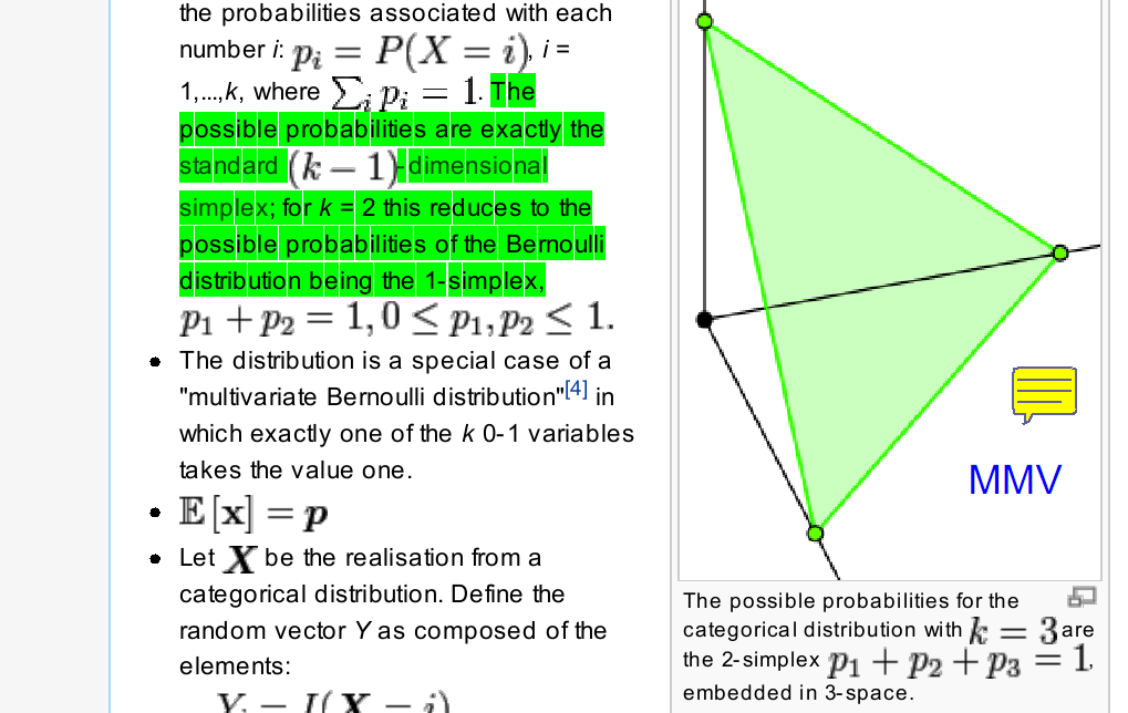
Мислам дека Cover со горното тврдење сака да каже дека p(X2) е дискретна дистрибуција и дека вредностите и веројатностите може така да се подредат така што се добива линеарна дистрибуција. Сеедно е дали изводот во Lagrange Multipliers е по pi или по i.
I(X1;Y|X2) = H(Y|X2) − H(Y|X1X2) = ∑p(x2)p(x2)H(Y|X2 = x2) + ∑p(x2)p(x2)H(Y|X1, X2 = x2)
Линеарноста потекнува од таму што p(x2) ги множи ентропиите во горниот израз. Се едно е дали во производот ќе стои p(x2) или само x2 кога ќе пресметуваш максимум со лагранжови множители.
Given any (M, n) code fort the relay channel, the probability mass function on the joint ensemble W, X1, X2, Y, Y1 is given by:
Ова не успеав да го докажам во целост!?
W → X1 → (X2, Y1) → Y
p(w, x1, y, y1, x2) = (1)/(M)⋅p(x1|w)⋅p(y, y1|x1w)⋅p(x2|x1w, y, y1) = (1)/(M)⋅p(x1|w)⋅p(y, y1|x1)⋅p(x2|x1, y, y1)
p(w, x1, y1, x2, y) = (1)/(M)⋅p(x1|w)⋅p(y1|w, x1)⋅p(x2|x1w, y1)⋅p(y, |(x1w), (x2, y1)) = (1)/(M)⋅p(x1|w)⋅p(y1|x1)⋅p(x2|y1)⋅p(y|x1x2) = (1)/(M)⋅p(x1|w)⋅p(x2|y1)⋅p(y1|x1)⋅p(y|x1x2)
p(w, x1, x2, y1, y) = (1)/(M)⋅p(x1|w)⋅p(x2|w, x1)⋅p(y1y|x1x2, w) = (1)/(M)⋅p(x1|w)⋅p(x2|x1)⋅p(y1y|x1x2)
X2 = f(Y1) → p(Y|X2, Y1) = p(Y|f(X2), Y1) = p(Y|Y1) слично X1 = f(W)
Вака размислувајќи излегува дека Марковиoт ланец можеш да го толкуваш преку функционална зависност на случајните промениви.
Нови моменти што произлегоа од подолните изведувања
By discrete memorylessness of the channel, Yi and (W, Yi − 1) are conditionaly independent given (X1i, X2i).
It is easy to see that W and X2i are conditionaly independent given (Yi − 1, Yi − 1).
18.06.14
Мислам дека нема што да се докажува по дефиниција x2 зависи од претходните примени симболи во релето.
p(W, Xn1, Xn2, Yn, Yn1) = (1)/(M)⋅p(Xn1|w)⋅p(Xn2|Xn1)⋅p(Yn, Yn1|Xn1, Xn2) = (1)/(M)⋅p(Xn1|w)⋅p(Xn2|Xn1)⋅p(Yn, Yn1|Xn1, Xn2)
= (1)/(M)⋅p(x1|w)⋅∏ni = 1p(x2i|x11, ..., x1i − 1)⋅p(yi, y1i|x1i, x2i)
Consider the identity
nR = H(W) = I(W;Y) + H(W|Y)
By Fano’s inequality
Thus
nR ≤ H(W) = I(W;Y) + H(W|Y) = I(W;Y) + nδn
We now upper bound
I(W;Y) in a lemma that is essentially similar to Theorem 10.1 in
[1].
Proof: To simplify notation, we shall use Yi = (Y1, Y2, ...Yi) throughout the rest of this paper. First considering i), we apply the chain rule to obtain.
I(W;Y) = n⎲⎳i = 1I(W;Yi|Yi − 1) = n⎲⎳i = 1(H(Yi|Yi − 1) − H(Yi|Yi − 1, W)) ≤
(a) во последното неравенство користи conditioning reduces entropy.
By discrete memorylessness of the channel, Yi and (W, Yi − 1) are conditionaly independent given (X1i, X2i).
I(W;Y) ≤ n⎲⎳i = 1(H(Yi) − H(Yi|X1iX2i)) = n⎲⎳i = 1I(X1i, X2i;Yi)
Considerig ii) we have
I(W;Y) ≤ I(W;Y, Y1) = I(W;Y) + I(W;Y1|Y) = n⎲⎳i = 1I(W;Yi, Y1i|Yi − 1Yi − 11) = n⎲⎳i = 1H(W|Yi − 1Yi − 11) − H(W|Yi, Y1i, Yi − 1, Yi − 11)
It is easy to see that W and X2i are conditionally independent given (Yi − 1, Yi − 11).
Претпоставувам се работи за марков ланец т.е. деградиран релеен канал каде W → (Y, Y1) → X2
Hence
and continuing the sequence of upper bounds in
49↑, we have
I(W;Y) ≤ n⎲⎳i = 1H(W|Yi − 1Yi − 11, X2i) − H(W|Yi, Yi1, X2i) = n⎲⎳i = 1I(W;Yi, Y1i|Yi − 11Yi − 1X2i) =
= n⎲⎳i = 1H(Yi, Y1i|Yi − 11Yi − 1X2i) − H(Yi, Y1i|\mathchoiceW, Yi − 11Yi − 1W, Yi − 11Yi − 1W, Yi − 11Yi − 1W, Yi − 11Yi − 1X2i)\overset(d) ≤ n⎲⎳i = 1H(Yi, Y1i|X2i) − H(Yi, Y1i|X1iX2i) = n⎲⎳i = 1I(X1i;YiY1i|X2i)
Не контам зошто ова во жолтово го менува со X1i? Можеби заради дефиницијата 43↑?
19.06.2014
(d) следи од следниве неравенсттва
∑ni = 1H(Yi, Y1i|Yi − 11Yi − 1X2i) − H(Yi, Y1i|W, Yi − 11Yi − 1X2i) ≤ ∑ni = 1H(Yi, Y1i|Yi − 11Yi − 1X2i) − H(Yi, Y1i|W, Yi − 11Yi − 1X1iX2i) ≤ (*)
Слично како во
48↑ од фактот дека се работи за дискретен канал без меморија,
YiY1i не зависат од
Yi − 1Yi − 11 ниту зависат од
W ако се дадени
(X1i, X2i).
(*) ≤ ∑ni = 1H(Yi, Y1i|Yi − 11Yi − 1X2i) − H(Yi, Y1i|X1iX2i) ≤ ≤ ∑ni = 1H(Yi, Y1i|X2i) − H(Yi, Y1i|X1iX2i) = ∑ni = 1I(X1i;Yi, Y1i|X2i)
And Lemma 4 is proved.
From
45↑ and Lemma 4 it follows that
R ≤ min⎧⎩(1)/(n)n⎲⎳i = 1I(X1i, X2i;Yi), (1)/(n)n⎲⎳i = 1I(X1i;Y1i, Yi|X2i)⎫⎭ + δn
19.06.14
Од Лема 4 се гледа дека
I(W;Y) е помало и од
∑ni = 1I(X1i, X2i;Yi) и од
∑ni = 1I(X1i;Y1i, Yi|X2i) логично дека ако ги ставиш во операција min дека повторно
I(W;Y) ќе биде помало од нив. На тој начин ги прави минимумите во теоремите 1, 2 и 3.
. Мислам дека ова изведување е убаво и може да влезе во Докторската.
We now eliminate the variable n by simple artifice. Let Z be random variable independent of X1X2, Y, Y1 taking values in the set {1, ...n}with probability:
X1≜X1Z, X2≜X2Z, Y≜YZ Y1≜Y1Z
Then
(1)/(n)n⎲⎳i = 1I(X1i, X2i;Yi) = I(X1, X2;Y|Z) ≤ I(X1, X2;Y)
Ова е класичен пристап за time sharing што на пример Cover го користи во Главата 15.3 за multiple access channel. Таму го имам и елеганто докажано.
потсетување за ентропија на disjoint mixture
p(X1) = {p1, p2...pn} p(X2) = {q1, q2...qn} θ = f(X) = ⎧⎨⎩
1
with probability p(X = X1) = α
2
with probability p(X = X2) = 1 − α
H(θ, X) = H(θ) + H(X|θ) = H(X) + \cancelto0H(θ|X) ⇒ H(X) = H(θ) + H(X|θ) = H(α) + p(θ = 0)⋅H(X|θ = 0) + p(θ = 1)⋅H(X|θ = 1)
= H(α) + α⋅H(X|θ = 0) + (1 − α)⋅H(X|θ = 1) = H(α) + α⋅H(p) + (1 − α)⋅H(q)
Ова може да се генерализира за повеќе од 2 индекси т.е. disjoint mixtures.
Потсетување на тотална експектација
E- коцката паднала на парен број
E(X|E) = 2⋅(1)/(3) + 4⋅(1)/(3) + 6⋅(1)/(3) = 4
E(X|E) = 1⋅(1)/(3) + 3⋅(1)/(3) + 5⋅(1)/(3) = 3
E(X) = p(E)⋅E(X|E) + p(E)⋅E(X|E) = 4 ⁄ 2 + 3 ⁄ 2 = 7 ⁄ 2
(1 + 2 + 3 + 4 + 5 + 6)/(6) = (7)/(2)
Доказ на изразот:
(1)/(n)∑2i = 1I(X1iX2i;Yi) = \cancelto(1)/(2)p(Z = 1)⋅I(X11X21;Y1) + \cancelto(1)/(2)p(Z = 2)⋅I(X12X22;Y2)
\mathchoiceI(X21X22;Y2|Z)I(X21X22;Y2|Z)I(X21X22;Y2|Z)I(X21X22;Y2|Z) = H(X11, X12X21, X22|Z) − H(X11X12X21, X22|Y1Y2, Z) = p(Z = 1)⋅H(X21X22|Z = 1) + p(Z = 2)H(X21X22|Z = 2)
− p(Z = 1)⋅H(X21X22|Y2, Z = 1) − p(Z = 2)⋅H(X21X22|Y2, Z = 2) = p(Z = 1)⋅H(X11X21) + p(Z = 2)⋅H(X12X22)
− p(Z = 1)⋅H(X11X21|Y1) − p(Z = 2)⋅H(X12X22|Y2) = p(Z = 1)⋅I(X11X21;Y1) + p(Z = 2)⋅I(X12, X22;Y12) = \mathchoice(1)/(n)∑ni = 1I(X1i, X21;Yi)(1)/(n)∑ni = 1I(X1i, X21;Yi)(1)/(n)∑ni = 1I(X1i, X21;Yi)(1)/(n)∑ni = 1I(X1i, X21;Yi) n = 2
Треба да го докажам и со користење на:
\strikeout off\uuline off\uwave offZ → (X1X2) → (Y, Y1)
\mathchoiceI(X21X22;Y2|Z)I(X21X22;Y2|Z)I(X21X22;Y2|Z)I(X21X22;Y2|Z) = H(X11, X12X21, X22|Z) − H(X11X12X21, X22|Y1Y2, Z) = H(Y1Y2|Z) − H(Y1Y2|X11, X12X21, X22, Z)
\mathchoiceI(X21X22;Y2|Z)I(X21X22;Y2|Z)I(X21X22;Y2|Z)I(X21X22;Y2|Z) = H(Y2|Z) − H(Y2|X21X22, Z) = H(Y2|Z) − H(Y2|X21X22) = p(Z = 1)⋅H(Y1) + p(Z = 2)⋅H(Y2) − H(Y1|X21X22) − \overset(a)H(Y2|Y1X21X22) =
(a) - W = f(X1) значи слободно можеш да го додадеш во условот нема да додаден никаква информација.
= p(Z = 1)⋅H(Y1) + p(Z = 2)⋅H(Y2) − H(Y1|X21X22) − \overset(b)H(Y2|Y1X21X22W) =
(b) - By discrete memorylessness of the channel, Yi and (W, Yi − 1) are conditionaly independent given (X1i, X2i).
= p(Z = 1)⋅H(Y1) + p(Z = 2)⋅H(Y2) − H(Y1|X21X22) − H(Y2|X21X22W) = p(Z = 1)⋅H(Y1) + p(Z = 2)⋅H(Y2) − H(Y1|X21X22) − H(Y2|X21X22) =
= p(Z = 1)⋅H(Y1) + p(Z = 2)⋅H(Y2) − H(Y1|X21X22) − H(Y2|X21X22W) =
\strikeout off\uuline off\uwave off = p(Z = 1)⋅H(Y1) + p(Z = 2)⋅H(Y2) − p(Z = 1)⋅H(Y1|X11X21) − p(Z = 2)⋅H(Y2|X12X22) = \mathchoice(1)/(n)∑ni = 1I(X1i, X21;Yi)(1)/(n)∑ni = 1I(X1i, X21;Yi)(1)/(n)∑ni = 1I(X1i, X21;Yi)(1)/(n)∑ni = 1I(X1i, X21;Yi) n = 2
19.06.2014
Мислам дека доказот во EIT Chapter 15.3.4 Notebook-т е поедноставен.
24.06.14
Марковата релација ја користат за докажување на последната нееднаквост
I(X1, X2;Y|Z) ≤ I(X1, X2;Y)
I(X1, X2;Y|Z) = H(Y|Z) − H(Y|Z, X1X2) ≤ H(Y) − H(Y|Z, X1, X2) = H(Y) − H(Y|X1, X2) = I(X1, X2;Y)
by the Markovian relation \mathchoiceZ → (X1X2) → (Y, Y1)Z → (X1X2) → (Y, Y1)Z → (X1X2) → (Y, Y1)Z → (X1X2) → (Y, Y1) induced by channel and the code. Similarly:
(1)/(n)n⎲⎳i = 1I(X1i;Yi, Y1i|X2i) = I(X1;Y, Y1|X2, Z) ≤ I(X1;Y, Y1|X2)
Thus
\mathchoiceR ≤ min{I(X1, X2;Y1), I(X1;Y, Y1|X2)} + δnR ≤ min{I(X1, X2;Y1), I(X1;Y, Y1|X2)} + δnR ≤ min{I(X1, X2;Y1), I(X1;Y, Y1|X2)} + δnR ≤ min{I(X1, X2;Y1), I(X1;Y, Y1|X2)} + δn
and Theorem 4 is proved.
Овој доказ е едноставен и добар. Може да влезе во PhD, без делот за achievability. Логично е зошто за да го определи капацитетот бара од овој израз потоа supremum по p(x1, x2). Затоа што капацитетот е супремум од сите достигливи брзини на пренесување.
4 The Gaussian DEGRADED Relay Channel(current)
Suppose a transmitter x1 with power P1 sends a signal intended for receiver y. However this signal is also received by a relay y1 that is perhaps physically closer to x1 than is to y. Transmissions are corrupted by additive Gaussian noise. How can the relay x2 make good use of y1 to send a signal at power P2 that will add to the signal received by the ultimate receiver y?
First we define the model for discrete time additive white Gaussian noise degraded relay channel as shown in
4↓.
Let Z1 = (Z11, ..., Z1n) be a sequence of independen identically distributed (i.i.d) normal random variables (r.v.’s) with mean zero and variance N1, and let Z2 = (Z21, ..., Z2n) be i.i.d normal r.v.’s independent of Z1 with mean zero and variance N2. Define N = N1 + N2. At the i-th transmission the real number x1i and x2i are sent and:
\mathchoicey1i = x1i + z1iy1i = x1i + z1iy1i = x1i + z1iy1i = x1i + z1i
\mathchoiceyi = x2i + y1i + ziyi = x2i + y1i + ziyi = x2i + y1i + ziyi = x2i + y1i + zi
are received. Thus the channel is degraded
\strikeout off\uuline off\uwave offp(y, y1|x1, x2) = p(y1|x1, x2)⋅p(y|y1, x2) сака да каже дека y не зависи од x1 ако се дадени (y1, x2)
.
Let the message power constraint on the transmitted power be:
and
for transmitted signal x1 = (x11, ..., x1n) and relay signal x2 = (x21, ..., x2n) respectively.
The definition of a code for this channel is the same as given in section I with the additional constraints in
52↑.
The capacity C* of the Gaussian degraded relay channel is given by:
where α = (1 − α) and:
C(X) = (1)/(2)⋅log(1 + x) x ≥ 0
Најдобра анализа од која потоа оваа лесно се конта е онаа за multi-access channel од EIT Chapter 15.3.6
1) If
(P2)/(N2) ≥ (P1)/(N1)
it can be seen that C* = C⎛⎝(P1)/(N1)⎞⎠(This is achieved by α = 1). The channel appears to be noise free after the relay, an the capacity C⎛⎝(P1)/(N1)⎞⎠ from the x1 to the relay can be achieved. Thus the rate without the relay C⎛⎝(P1)/(N1 + N2)⎞⎠ is increased by the relay to C⎛⎝(P1)/(N1)⎞⎠. For large N2, and for \strikeout off\uuline off\uwave off(P2)/(N2) ≥ (P1)/(N1) we see that the increment in rate is from C⎛⎝(P1)/(N1 + N2)⎞⎠\thickapprox0 to C⎛⎝(P1)/(N1)⎞⎠.
2) For (P2)/(N2) < (P1)/(N1), it can be seen that the maximizing α = α* is strictly less that one, and is given by solving for α in:
ln⎛⎝(P1 + P2 + 2⋅√(αP1P2))/(N)⎞⎠ = ln⎛⎝1 + (αP1)/(N1)⎞⎠
yielding C* = C⎛⎝α*(P1)/(N1)⎞⎠.
\undersetfln⎛⎝1 + (P1 + P2 + 2⋅√(αP1P2))/(N)⎞⎠ = \undersetgln⎛⎝1 + (αP1)/(N1)⎞⎠
(N1P2)/(N2) < P1 P2 < (N2P1)/(N1)
(P1 + P2 + 2⋅√(αP1P2))/(N) = 1 + (αP1)/(N) (P1 + P2 + 2⋅√(αP1P2))/(N) = (P1 + P2)/(N1 + N2) + (2√((1 − α)P2P1))/(N1 + N2) < (P1 + (N2P1)/(N1))/(N1 + N2) + (2√((1 − α)P1(N2P1)/(N1)))/(N1 + N2) = ((\cancel(N1 + N2)P1)/(N1))/(\cancelN1 + N2) + (2P1√((1 − α)(N2)/(N1)))/(N1 + N2) = (P1)/(N1) + (2P1)/(N1 + N2)√((1 − α)(N2)/(N1))
|α = 0| ≤ (P1)/(N1) + (2P1)/(N1 + N2)√((N2)/(N1))
Нешто се мотав ама овде не баш сваќам што сака да каже.
Еве сега при пофторното читањена PhD да го пререшам
ln⎛⎝1 + (P1 + P2 + 2⋅√(αP1P2))/(N)⎞⎠ = ln⎛⎝1 + (αP1)/(N1)⎞⎠
(P1 + P2 + 2⋅√(αP1P2))/(N) = 1 + (αP1)/(N) → Maple → \mathnormal[(P1 − P2 − N + 2 √(P2N))/(P1),(P1 − P2 − N − 2 √(P2N))/(P1)], [1-(P2 + N − 2 √(P2N))/(P1),1-(P2 + N + 2 √(P2N))/(P1)]
First we sketch the achievability of C* and the random code that achieves it. For 0 ≤ α ≤ 1 let \mathchoiceX2 ~ N(0, P2)X2 ~ N(0, P2)X2 ~ N(0, P2)X2 ~ N(0, P2), \mathchoiceX10 ~ N(0, αP1)X10 ~ N(0, αP1)X10 ~ N(0, αP1)X10 ~ N(0, αP1), with X10, X2 independent, and let
\mathchoiceX1 = √(α⋅(P1)/(P2))X2 + X10X1 = √(α⋅(P1)/(P2))X2 + X10X1 = √(α⋅(P1)/(P2))X2 + X10X1 = √(α⋅(P1)/(P2))X2 + X10. Then referring to Theorem 1, we evaluate:
I(X1, X2;Y) = ln⎛⎝(P1 + P2 + 2⋅√(αP1P2))/(N)⎞⎠
I(X1;Y1|X2) = (1)/(2)⋅ln⎛⎝1 + (αP1)/(N)⎞⎠
************************************************************************************************
X1 = √(α⋅(P1)/(P2))X2 + X10
EX21 = αP1 + αP1 = P1
X2 ~ N(0, P2), X10 ~ N(0, αP1)
y1i = x1i + z1i
yi = x2i + y1i + zi = x2i + x1i + z1i + zi
I(X1, X2;Y) = H(Y) − H(Y|X1X2) = H(X2 + Y1 + Z) − H(X2 + Y1 + Z|X1X2) =
= H(X2 + X1 + Z1 + Z) − H(X2 + X1 + Z1 + Z|X1X2) = (1)/(2)log(P2 + P1 + N1 + N2) − (1)/(2)log(N1 + N2) = (1)/(2)log(P1 + P2 + N1 + N2)/(N1 + N2) =
(1)/(2)log⎛⎝1 + (P1 + P2)/(N1 + N2)⎞⎠ = C⎛⎝1 + (P1 + P2)/(N1 + N2)⎞⎠
I(X1;Y1|X2) = H(X1 + Z1|X2) − H(X1 + Z1|X1X2) =
= H(X1 + Z1) − H(Z1) = (1)/(2)log(P1 + N1) − (1)/(2)log(N1) = (1)/(2)log(P1 + N1)/(N1 + N2) =
(1)/(2)log⎛⎝1 + (P1)/(N1)⎞⎠ = C⎛⎝(P1)/(N1)⎞⎠
Ако земеш P1 = αP1 следи
I(X1;Y1|X2) = C⎛⎝(αP1)/(N1)⎞⎠
***********************************************************************************************
Вака резонирам. Со оглед на тоа што I(X1;Y1|X2) е информацијата што се пренесува во претходниот тајмслот према релето тогаш снагата на X1 = X10
————————————————————
Потсетување од EIT Chapter 15.3.3
I(X2;Y|X1) = H(X2|X1) − H(X2|Y, X1) = H(X2) − H(X2|Y, X1) = I(X2;Y, X1) = I(X2;Y) + I(X2;X1|Y) ≥ I(X2;Y)
————————————————————–
\mathchoiceI(X1;Y1|X2)I(X1;Y1|X2)I(X1;Y1|X2)I(X1;Y1|X2) = H(X1 + Z1|X2) − H(X1 + Z1|X1X2) =
= H(X10 + Z1) − H(Z1) = (1)/(2)log(αP1 + N1) − (1)/(2)log(N1) = (1)/(2)log(P1 + N1)/(N1) = (1)/(2)log⎛⎝1 + (αP1)/(N1)⎞⎠ = \mathchoiceC⎛⎝(αP1)/(N1)⎞⎠C⎛⎝(αP1)/(N1)⎞⎠C⎛⎝(αP1)/(N1)⎞⎠C⎛⎝(αP1)/(N1)⎞⎠
I(X1;Y1|X2) + I(X2;Y) =
I(X1X2;Y) = I(X2;Y) + I(X1;Y|X2) = I(X2;Y) + H(Y|X2) − H(Y|X1X2)
I(X1;Y|X2) = H(Y|X2) − H(Y|X1X2) ≤ H(Y|X2) − H(Y|X1X2Y1) = (*)
H(Y|X1X2Y1) = H(Y|X2Y1)
(*) = H(Y|X2) − H(Y|X2Y1) = I(X2;Y|Y1) ≤ I(Y1;Y) + I(X2;Y|Y1) = I(X2Y1;Y)
For degraded channel we have:
X1 → (X2, Y1) → Y
I(X1;X2Y1) ≥ I(X1;Y)
\overset0I(X1;X2) + I(X1;Y1|X2) ≥ I(X1;Y) → \mathchoiceI(X1;Y1|X2) ≥ I(X1;Y)I(X1;Y1|X2) ≥ I(X1;Y)I(X1;Y1|X2) ≥ I(X1;Y)I(X1;Y1|X2) ≥ I(X1;Y)
************************************************************************************************
I(X1, X2;Y) = ln⎛⎝(P1 + P2 + 2⋅√(αP1P2))/(N)⎞⎠
E(X22) = P2((1 − √(α)))/((1 + √(α)))
y1i = x1i + z1i
yi = x2i + y1i + zi = x2i + x1i + z1i + zi
I(X1, X2;Y) = H(Y) − H(Y|X1X2) = H(X2 + Y1 + Z) − H(X2 + Y1 + Z|X1X2) =
= H(X2 + X1 + Z1 + Z) − H(X2 + X1 + Z1 + Z|X1X2) = (1)/(2)log⎛⎝P2((1 − √(α)))/((1 + √(α))) + P1 + N1 + N2⎞⎠ − (1)/(2)log(N1 + N2) = (1)/(2)log(P1 + P2 + N1 + N2)/(N1 + N2) =
****************************************************************************************************
The assertion that this distribution p(x1, x2) actually maximizes min{I(X1;Y1|X2), I(X1, X2;Y)} will follow from the proof of the converse.
The random codebook (Section II) associated with this distribution is then given by a random choice of:
X1̃(w) i.i.d. ~ Nn(0, αP1I) w ∈ [1, 2nR]
X2̃(s) i.i.d. ~ Nn(0, P2I) w ∈ [1, 2nR0]
\mathchoiceR0 = (1)/(2)log⎛⎝1 + ((√(P2) + √(αP1))2)/((αP1 + N))⎞⎠ − ϵ, R0 = (1)/(2)log⎛⎝1 + ((√(P2) + √(αP1))2)/((αP1 + N))⎞⎠ − ϵ, R0 = (1)/(2)log⎛⎝1 + ((√(P2) + √(αP1))2)/((αP1 + N))⎞⎠ − ϵ, R0 = (1)/(2)log⎛⎝1 + ((√(P2) + √(αP1))2)/((αP1 + N))⎞⎠ − ϵ, and Nn(0, I) denotes the n-variate normal distribution with identity co variance matrix I. The code book is given by
Немам идеја од каде го добива овој израз за R0. Претпоставувам нешто со пресметка на матрицата на коварианси. Ама како изгледа таа:
x1(w|s) = x1̃(w) + √((αP1)/(P2))x2(s)
x2(s), w ∈ [1, 2nR] s ∈ [1, 2nR0].
The codewords so generated (1 − ϵ)-satisfy the power constraints with high probability, and thus the overall average probability of error can be shown to be small.
Ова се неуспешните обиди да го најдам R0. Решението е во наредниот box.
I(X1, X2;Y) = ln⎛⎝(P1 + P2 + 2⋅√(αP1P2))/(N)⎞⎠
\strikeout off\uuline off\uwave offR0 = (1)/(2)log⎛⎝1 + ((√(P2) + √(αP1))2)/((αP1 + N))⎞⎠ − ϵ
\strikeout off\uuline off\uwave offX1 = √(α⋅(P1)/(P2))⋅X2 + X10
R0 ≤ I(X2;Y) = H(X2) − H(X2|Y)
R0 ≤ (1)/(2)log(2πe)⋅(σ2x2 + σ2Z2) − (1)/(2)log(2πe)⋅(σ2Z2) = (1)/(2)log(2πe)⋅(1 + (σ2x2)/(σ2Z2))
X2 = √((P2)/(αP1))(X1 − X10) E(X22) = (P2)/(αP1)⋅E((X1 − X10)2) ≤ P2
********************************************************************************
20.06.14
E((X1 − X10)2) = E(X21) − 2E(X1X10) + E(X20) = P21 − 2P1αP1 + α2P21
(P2)/(αP1)(P1 − 2√(P1)√(αP1) + αP1) = ⎛⎝(P2)/(1 − α) − (2√(α))/((1 − α))P2 + (α)/((1 − α))⋅P2⎞⎠ = (P2 − 2√(α)P2 + αP1)/((1 − α)) = (P2 − 2√(α)P2 + αP2)/((1 − α)) = P2((1 − √(α))2)/(1 − α) = P2((1 − √(α))\cancel2)/(\cancel(1 − √(α))(1 + √(α))) = P2((1 − √(α)))/((1 + √(α)))
E(X21) = E(√(α⋅(P1)/(P2))⋅X2 + X10)2 = P1 + 2√(α⋅(P1)/(\cancelP2))√(\cancelP2)√(αP1) + αP1 = P1 + 2√(ααP1P1) + αP1
Y = X1̂ + X2 E(X1̂2) = αP1
I(X1, X2;Y) = H(Y) − H(Y|X1X2) = H(X2 + X1 + Z) − H(X2 + X1 + Z|X1X2) =
= H(X2 + X1 + Z1 + Z) − H(Z1 + Z|X1X2) = (1)/(2)log(E(X1 + X2)2 + N1 + N2) − (1)/(2)log(N1 + N2) = (*)
E(X1 + X2)2 = αP1 + 2√(P1αP2) + P2
(*) = (1)/(2)log⎛⎝1 + (αP1 + 2√(P1αP2) + P2)/(N1 + N2)⎞⎠
**********************************************************************************
08.10.2014 (Овде више ги сменив ознаките во докторатот и се прилагодив на ознаките во NIT на El Gammal
Y3 = X2 + Y2 + Z3 = X2 + X1 + Z2 + Z3
R0 = I(X2;Y3) = (1)/(2)⋅log(Var[X2 + Y2 + Z3]) − (1)/(2)⋅log(Var[X2 + Y2 + Z3]|X2) = (1)/(2)⋅log(P2 + E(Y22) + N3) − (1)/(2)⋅log(E(Y22) + N3)
Изгледа зема Y2 ~ X10 ~ N(0, αP1) и претпоставува дека X2 е корелирано со Y2
R0 = I(X2;Y3) = (1)/(2)⋅log(Var[X2 + Y2 + Z3]) − (1)/(2)⋅log(Var[X2 + Y2 + Z3]|X2) = (1)/(2)⋅log(Var[X2 + X10 + Z2] + N3) − (1)/(2)⋅log(Var[αP1 + Z2 + Z3]) =
= (1)/(2)⋅log(Var[X2 + X10] + N2 + N3) − (1)/(2)⋅log(Var[X10] + N2 + N3) = (1)/(2)⋅log(Var[X2 + X10] + N) − (1)/(2)⋅log(Var[X10] + N) =
X1 = √(α⋅(P1)/(P2))⋅X2 + X10 → X10 = X1 − √(α⋅(P1)/(P2))⋅X2 → X2 = √((P2)/(αP1))⋅(X1 − X10)
E[X21] = (√(α⋅(P1)/(P2)))2⋅E[X22] + αP1 = α⋅(P1)/(P2)⋅P2 + αP1 = α⋅P1⋅ + αP1 = P1
Var[X2 + X1] = Var[X2 + √(α⋅(P1)/(P2))⋅X2 + X10] = P2 + (1 − α)P1 + αP1 = P2 + P1
Var[X2 + X1] = P2 + 2⋅E[X1X2] + P1 = P2 + 2⋅E[(√(α⋅(P1)/(P2))⋅X2 + X10)X2] + P1 = P2 + 2⋅E[√(α⋅(P1)/(P2))⋅X22 + X10X2] + P1 = P2 + 2⋅P2 + 2⋅E[X10X2] + P1 =
= P2 + 2⋅P2 + 2⋅αP1P2 + P1 = P2 + 2⋅P2 + 2⋅(1 − α)P1P2 + P1
(√(P2) + √(αP1))2 = P2 + 2√(αP1P2) + αP1
Var[X2 + X10] = P2 + 2⋅E[X10X2] + P1 = P2 + 2E[(X1 − √(α⋅(P1)/(P2))⋅X2)⋅X2] + P1 = P2 + 2⋅E[X1X2 − √(α⋅(P1)/(P2))⋅X2⋅X2] + P1 = P2 + 2√(P1)√(P2) − (1 − α)P1 + P1 = P2 + 2P1P2 + αP1
= P2 + 2P1P2 + (1 − α)P1 = P2 + 2P1P2 + P1 − αP1 + αP1 − αP1 = αP1 + P2 + 2P1P2 + P1 − \cancelαP1 − (1 − \cancelα)P1
(1)/(2)⋅log(Var[X2 + X10] + N) − (1)/(2)⋅log(Var[X10] + N) = (1)/(2)⋅log(Var[X2] + Var[X10] + N) − (1)/(2)⋅log(Var[X10] + N) = (1)/(2)⋅log⎛⎝(Var[X2])/(Var[X10] + N) + 1⎞⎠ =
= (1)/(2)⋅log⎛⎝(Var[X2])/(αP1 + N) + 1⎞⎠ X2 = √((P2)/(αP1))⋅(X1 − X10) Var[X2] = (P2)/(αP1)⋅(P1 − 2⋅E[X10X1] + αP1) = (P2)/(αP1)⋅(P1 − 2⋅E[α⋅X1X1] + αP1) = (P2)/(αP1)⋅(P1 − 2⋅α⋅P1 + αP1) = P2
Y3 = X2 + Y2 + Z3 = X2 + X1 + Z2 + Z3
X1 = √(α⋅(P1)/(P2))⋅X2 + X10 → X10 = X1 − √(α⋅(P1)/(P2))⋅X2 → X2 = √((P2)/(αP1))⋅(X1 − X10)
R0 = I(X2;Y3) = (1)/(2)⋅log(Var[X2 + Y2 + Z3]) − (1)/(2)⋅log(Var[X2 + Y2 + Z3]|X2) = (1)/(2)⋅log(Var[X2 + X10 + Z2] + N3) − (1)/(2)⋅log(Var[αP1 + Z2 + Z3]) =
= (1)/(2)⋅log(Var[X2 + X10] + N2 + N3) − (1)/(2)⋅log(Var[X10] + N2 + N3) = (1)/(2)⋅log(Var[X2 + X10] + N) − (1)/(2)⋅log(αP1 + N) =
Кога не би биле корелирани
R0 = (1)/(2)⋅log(P2 + αP1 + N) − (1)/(2)⋅log(αP1 + N) = (1)/(2)⋅log⎛⎝(P2)/((αP1 + N)) + 1⎞⎠
Ако се корелирани (а во чланакот велат дека не се) се добива:
Var[X2 + X10] = P2 + 2⋅E[X10X2] + P1 = P2 + 2E[(X1 − √(α⋅(P1)/(P2))⋅X2)⋅X2] + P1 = P2 + 2⋅E[X1X2 − √(α⋅(P1)/(P2))⋅X2⋅X2] + P1 = P2 + 2√(P1)√(P2) − (1 − α)P1 + P1 = P2 + 2√(P1)√(P2) + αP1
R0 = (1)/(2)⋅log(P2 + 2√(P1)√(P2) + αP1 + N) − (1)/(2)⋅log(αP1 + N) = (1)/(2)⋅log⎛⎝(P2 + 2√(P1)√(P2))/((αP1 + N)) + 1⎞⎠
X1 = √(α⋅(P1)/(P2))⋅X2 + X10 → X10 = X1 − √(α⋅(P1)/(P2))⋅X2 → X2 = √((P2)/(αP1))⋅(X1 − X10)
R0 = I(X2;Y3) = (1)/(2)⋅log(Var[X2 + Y2 + Z3]) − (1)/(2)⋅log(Var[X2 + Y2 + Z3]|X2) = (1)/(2)⋅log(Var[X2 + X1 + Z2 + Z3]) − (1)/(2)⋅log(Var[X1 + Z2 + Z3]|X2) =
= (1)/(2)⋅log(Var[X2 + X1] + N) − (1)/(2)⋅log(Ex2{Var[X1|X2]} + N)
\mathchoiceEx2{Var[X1|X2]}Ex2{Var[X1|X2]}Ex2{Var[X1|X2]}Ex2{Var[X1|X2]} = E[X21] − (E[X1X2])/(E[X22]) = P1 − (E2[(√(α⋅(P1)/(P2))⋅X2 + X10)X2])/(P2) = P1 − (E2[√(α⋅(P1)/(P2))⋅X22] + \cancelto0E[X10X2])/(P2) = P1 − (α(P1)/(P2)⋅P22)/(P2) = P1 − (αP1⋅P2)/(P2) = P1 − αP1 = \mathchoiceαP1αP1αP1αP1
Гледаш сега од каде излегува
αP1!!!
R0 = (1)/(2)⋅log(Var[X2 + X1] + N) − (1)/(2)⋅log(αP1 + N) = (1)/(2)⋅log((Var[X2 + X1] + N))/(αP1 + N)
Var[X2 + X1] = P2 + 2⋅E[X1X2] + P1 = P2 + 2⋅E[(√(α⋅(P1)/(P2))⋅X2 + X10)X2] + P1 = P2 + 2⋅E[√(α⋅(P1)/(P2))⋅X22 + X10X2] + P1 = P2 + 2⋅√(α⋅(P1)/(P2))⋅P2 + 2⋅\cancelto0E[X10X2] + P1 =
P2 + 2⋅√(α⋅P1P2) + P1 = P2 + 2⋅√(α⋅P1P2) + αP1 + αP1
R0 = (1)/(2)⋅log((P2 + 2⋅√(α⋅P1P2) + αP1 + αP1 + N))/(αP1 + N) = (1)/(2)⋅log⎛⎝1 + ((P2 + 2⋅√(α⋅P1P2) + αP1))/(αP1 + N)⎞⎠ = (1)/(2)⋅log⎛⎝1 + ((√(P2) + √(αP1))2)/(αP1 + N)⎞⎠
(√(P2) + √(αP1))2 = P2 + 2√(αP1P2) + αP1
Q.E.D!!!
Now the converse. Any code for the channel specifies a joint probability distribution W, X1, X2, Y1, Y.
nR ≤ n⎲⎳i = 1I(X1i;Y1i, Yi|X2i) + nδn = n⎲⎳i = 1I(X1i;Y1i|X2i) + nδn
From corollary 1:I(X1;Y, Y1|X2) = I(X1;Y1|X2)
by degradedness. Thus
nR ≤ n⎲⎳i = 1[H(Y1i|X2i) − H(Y1i|X2i, X1i)] + nδn = n⎲⎳i = 1[H(Y1i|X2i) − H(X1i + Z1i|X2i, X1i)] + nδn
= n⎲⎳i = 1[H(Y1i|X2i) − n⎲⎳j = 1p(X1i = x1j)H(x1j + Z1i|X2i, X1i = x1j)] + nδn = n⎲⎳i = 1[H(Y1i|X2i) − H(Z1i|X2i)] + nδn =
Now for any i:
Y1i = X1i + Z1i then
E[var(Y1i|X2i)] = E[E((X1i + Z1i)2 − (X1i + Z1i)2|X2i)] = |E[X1iZ1i] = 0| = E[var(X1i|X2i)] + E[Z21i] = Ai + N1
where
E[var(X1i|X2i)] = Ai, i = 1..n . Substituting in
55↑ we have:
again by Jensen’s inequality. However
\mathchoice(1)/(n)n⎲⎳i = 1Ai(1)/(n)n⎲⎳i = 1Ai(1)/(n)n⎲⎳i = 1Ai(1)/(n)n⎲⎳i = 1Ai = (1)/(n)n⎲⎳i = 1(E(X21i) − E(E2(X1|X2i))) ≤ P1 − \mathchoice(1)/(n)n⎲⎳i = 1EE2(X1i|X2i)(1)/(n)n⎲⎳i = 1EE2(X1i|X2i)(1)/(n)n⎲⎳i = 1EE2(X1i|X2i)(1)/(n)n⎲⎳i = 1EE2(X1i|X2i)
Ai = Ex2[var(X1i|X2i)] = EX2(EX1(X21i|X2i) − E2X1(X1i|X2i)) = EX1(X21i) − EX2E2X1(X1i|X2i)
Ова следи од total Expectation theorem.
by the power constraint on the code book.
Define:
R ≤ (1)/(2)⋅ln2πe⎛⎝1 + (P1 − αP1)/(N1)⎞⎠ + δn = (1)/(2)⋅ln2πe⎛⎝1 + (P1 − (1 − α)P1)/(N1)⎞⎠ + δn = (1)/(2)⋅ln2πe⎛⎝1 + (αP1)/(N1)⎞⎠ + δn.
Многу убави и елегантни работи има во овој доказ! Би рекол дека се работи за суштински изведувања!!!
\strikeout off\uuline off\uwave off
y1i = x1i + z1i
nR ≤ n⎲⎳i = 1I(X1i, X2i;Yi) + nδn ≤ n⎲⎳i = 1[H(Yi) − H(Yi|X1iX2i)] + nδn = n⎲⎳i = 1[H(X2i + Y1i + Zi) − H(X2i + Y1i + Zi|X1iX2i)] + nδn =
n⎲⎳i = 1[H(X2i + Y1i + Zi) − H(X2i + X1i + Z1i + Zi|X1iX2i)] + nδn = n⎲⎳i = 1[H(X2i + Y1i + Zi) − H(Z1i + Zi)] + nδn =
n⎲⎳i = 1⎡⎣H(X2i + Y1i + Zi) − (1)/(2)log(2πe)\oversetN(N1 + N2)⎤⎦ + nδn = n⎲⎳i = 1⎡⎣H(X2i + X1i + Z1i + Zi) − (1)/(2)log(2πe)N⎤⎦ + nδn =
for any i,
Hence
\mathchoiceRRRR ≤ (1)/(n)⋅n⎲⎳i = 1(1)/(2)ln2πe(E(X1i + X2i)2 + N) − (1)/(2)log(2πe)N = (1)/(n)⋅n⎲⎳i = 1(1)/(2)ln⎛⎝1 + (E(X1i + X2i)2)/(N)⎞⎠ + δn ≤
≤ (1)/(2)ln⎛⎝1 + (\mathchoice(1)/(n)⋅n⎲⎳i = 1E(X1i + X2i)2(1)/(n)⋅n⎲⎳i = 1E(X1i + X2i)2(1)/(n)⋅n⎲⎳i = 1E(X1i + X2i)2(1)/(n)⋅n⎲⎳i = 1E(X1i + X2i)2)/(N)⎞⎠ + δn.
EX1X2(X1X2) = |p(x1x2) = p(x2)⋅p(x1|x2)| = ∫∞ − ∞∫∞ − ∞x1x2p(x2)⋅p(x1|x2)dx1dx2 = ∫∞ − ∞x2p(x2)(\oversetEX1[X1|X2]∫∞ − ∞x1⋅p(x1|x2)dx1)dx2
= EX2[X2⋅EX1[X1|X2]] = E[X2⋅E[X1|X2]] ≤
√(∫∞ − ∞\mathchoicex22x22x22x22⋅p(x2)dx2⋅∫∞ − ∞\mathchoice(∫∞ − ∞x1p(x1|x2)dx1)2(∫∞ − ∞x1p(x1|x2)dx1)2(∫∞ − ∞x1p(x1|x2)dx1)2(∫∞ − ∞x1p(x1|x2)dx1)2p(x2)dx2) = √(E[X22]⋅E{E2[X1i|X2i]})
|∫ℜnf(x)⋅g(x)dx|2 ≤ ∫Rn\mathchoice|f(x)|2|f(x)|2|f(x)|2|f(x)|2dx⋅∫Rn\mathchoice|g(x)|2|g(x)|2|g(x)|2|g(x)|2dx
Applying the Cauchy Schwartz inequality to each term in the sum in
60↑, we obtain
The Cauchy-Schwattz inequality states that for all vectors x and y of an inner product space it is true that
|⟨x, y⟩|2 ≤ ⟨x, x⟩⋅⟨y, y⟩ |⟨x, y⟩| ≤ ∥x∥⋅∥y∥;
In Euclidean space ℜn with the standard inner product the Cauchy-Schwartz inequality is:
(∑ni = 1xiyi)2 ≤ (∑ni = 1x2i)⋅(∑ni = 1y2i)
(⟨⟨a, b⟩, ⟨c, d⟩⟩2) = = (ac + bd)2 = a2c2 + 2acbd + b2d2 ≤ (a2 + b2)⋅(c2 + d2) = a2c2 + a2d2 + b2c2 + b2d2
For the inner product space of square-integrable compex-valued functions, one has
|∫ℜnf(x)⋅g(x)dx|2 ≤ ∫Rn|f(x)|2dx⋅∫Rn|g(x)|2dx
-Апликација на шварцовото неравенство во теорија на веројатност:
In fact we can define an inner product on the set of random variables using the expectation of their product:
\mathchoice⟨X, Y⟩≜E(XY)⟨X, Y⟩≜E(XY)⟨X, Y⟩≜E(XY)⟨X, Y⟩≜E(XY)
And so the cauchy-Schwartz inequality,
|E(XY)|2 ≤ E(X2)E(Y2)
Moreover, if μ = E(X) and ν = E(Y), then
|Cov(X, Y)|2 = |E((X − μ)(Y − ν))|2 = |⟨X-μ, Y − ν⟩|2 ≤ ⟨X-μ, X − ν⟩⟨X-μ, Y − ν⟩ = E((X − μ)2)E((Y − ν)2) = Var(X)⋅Var(Y)
Значи коваријансата е помала од производот на поединечните варијанси на случајните променливи.
\mathchoice|Cov(X, Y)|2 ≤ Var(X)⋅Var(Y)|Cov(X, Y)|2 ≤ Var(X)⋅Var(Y)|Cov(X, Y)|2 ≤ Var(X)⋅Var(Y)|Cov(X, Y)|2 ≤ Var(X)⋅Var(Y)
\mathchoice(1)/(n)⋅n⎲⎳i = 1E(X1i + X2i)2(1)/(n)⋅n⎲⎳i = 1E(X1i + X2i)2(1)/(n)⋅n⎲⎳i = 1E(X1i + X2i)2(1)/(n)⋅n⎲⎳i = 1E(X1i + X2i)2 ≤ P1 + P2 + \mathchoice(2)/(n)n⎲⎳i = 1√(E[X22i]⋅E{E2[X1i|X2i]})(2)/(n)n⎲⎳i = 1√(E[X22i]⋅E{E2[X1i|X2i]})(2)/(n)n⎲⎳i = 1√(E[X22i]⋅E{E2[X1i|X2i]})(2)/(n)n⎲⎳i = 1√(E[X22i]⋅E{E2[X1i|X2i]})
From
58↑ and the power constraints we know that
n⎲⎳i = 1EE2(X1i|X2i) = αP1 (1)/(n)n⎲⎳i = 1E[X22i] ≤ P2
Again applying the Cauchy-Schwartz inequality, we have
\mathchoice2n⎲⎳i = 1⎛⎝(E[X22i])/(n)⎞⎠1 ⁄ 2⎛⎝(E{E2[X1i|X2i]})/(n)⎞⎠1 ⁄ 2 ≤ √((αP1)P2)2n⎲⎳i = 1⎛⎝(E[X22i])/(n)⎞⎠1 ⁄ 2⎛⎝(E{E2[X1i|X2i]})/(n)⎞⎠1 ⁄ 2 ≤ √((αP1)P2)2n⎲⎳i = 1⎛⎝(E[X22i])/(n)⎞⎠1 ⁄ 2⎛⎝(E{E2[X1i|X2i]})/(n)⎞⎠1 ⁄ 2 ≤ √((αP1)P2)2n⎲⎳i = 1⎛⎝(E[X22i])/(n)⎞⎠1 ⁄ 2⎛⎝(E{E2[X1i|X2i]})/(n)⎞⎠1 ⁄ 2 ≤ √((αP1)P2)
Во овој случај се користи класичното Шварцово неравенство:
(∑ni = 1xiyi)2 ≤ (∑ni = 1x2i)⋅(∑ni = 1y2i)2
⎛⎝∑ni = 1⎛⎝2⋅(E[X22i])/(n)⎞⎠1 ⁄ 2⎛⎝2⋅(E{E2[X1i|X2i]})/(n)⎞⎠1 ⁄ 2⎞⎠2 ≤ ∑ni = 1⎛⎝2⋅(E[X22i])/(n)⎞⎠∑ni = 1⎛⎝2⋅(E{E2[X1i|X2i]})/(n)⎞⎠
⎛⎝∑ni = 1⎛⎝2⋅(E[X22i])/(n)⎞⎠1 ⁄ 2⎛⎝2⋅(E{E2[X1i|X2i]})/(n)⎞⎠1 ⁄ 2⎞⎠ ≤ √(∑ni = 1⎛⎝2⋅(E[X22i])/(n)⎞⎠⋅∑ni = 1⎛⎝2⋅(E{E2[X1i|X2i]})/(n)⎞⎠) = 2⋅√((1)/(n)∑ni = 1E[X22i]⋅(1)/(n)∑ni = 1E{E2[X1i|X2i]}) = 2⋅√(P2(αP1))
Where the maximum occurs when \strikeout off\uuline off\uwave offE{E2[X1i|X2i]} = αP1 and E[X22i] = P2 for all i. Therefore
Converse follows directly form
58↑ and
61↑.
5 The capacity of the General Relay Channel with Feedback (current)
Suppose we have a relay channel
(X1xX2, p(y, y1|x1x2), Y1 Y2). No degradedness relation between
y and
y1 will be assumed.
Let there be feedback from (y, y1) to x1 and to x2 as shown in 5↓.
to be precise the encoding functions in
2↑ and
3↑ now become
x1i(w, y1, y2..., yi − 1, y11y12..., y1i − 1)
Placing a distribution on
w ∈ [1, 2nR] thus induces the joint probability mass function.
where yk = (y1, y2, ..., yk). Theorem 3 states that the capacity CFB of this channel is:
The relay channel with feedback is ordinary degraded relay channel under the substitution of (Y, Y1) for Y1. Thus the code and proof of the forward part of Theorem 1 apply, yielding the
ϵ-achievability of
CFB. For this converse, inspection of the proof of Theorem 4 reveals that all the steps apply to the feedback channel - the crucial step being
50↑. Thus the proof of Theorem 3 is complete.
The code used in Theorem 1 will suffice for the feedback channel. However, this code can be simplified by eliminating the random partitions
S, because the relay knows the
y sequence through the feedback link. An enumeration encoding for the relay can be used instead
[6].
If the channel (X1xX2, p(y, y1|x1x2), YxY1) is degraded or reversely degraded then feedback does not increase the capacity.
If the channel is degraded, then
I(X1;Y, Y1|X2) = I(X1;Y1|X2)
Thus CFB = C. If the channel is reversely degraded, then
I(X1;Y, Y1|X2) = I(X1;Y|X2)
Thus CFB = C.
6 An achievable Rate for the General Relay Channel
We are now in a position to discuss the nature of the capacity region for the general relay channel. First, if we have feedback we know the capacity. Next, we note that the general relay channel will involve the idea of cooperation (for the degraded relay channel) and facilitation (for the reversely degraded relay channel). If y1 is better than the y, then the relay cooperates to send x1; if y1 is worse than y, then the relay facilitates the transmission of x1 by sending the best x2. Yet another consideration will undoubtedly be necessary - the idea of sending alternative information. This alternative information about x1 is not zero, thus precluding simple facilitation, and is not perfect, thus precluding pure cooperation.
Finally, we note that the converse (Theorem 4) yields:
Cgeneral ≤ maxp(x1x2){I(X1, X2;Y), I(X1;Y, Y1|X2)}
For the general channel. Moreover, the code construction for Theorem 1 shows that
Cgeneral ≥ maxp(x1x2){I(X1, X2;Y), I(X1;Y1|X2)}
Also, from Theorem 2, we see
Cgeneral ≥ maxp(x1)maxx2I(X1;Y|x2).
If the relay channel is not degraded, cooperation may not be possible and facilitation can be improved upon. As an example consider the general Gaussian relay channel shown in Fig. 5.
If we assume that \mathchoiceN1 > NN1 > NN1 > NN1 > N, then cooperation in the sense of Section II cannot be realized, since every (2nR, n, ϵ) code for y1 will be a (2nR, n, ϵ) code for y. However, the relay sequence Y1 is an „observation” of X1 that is independent of Y. Thus sending Y1 to y will decrease the effective noise in the y observation of x1. If the relay power P1 is finite, and therefore we cannot sent Y1 to y precisely, then we send an estimate Ŷ1 of Y1.
Мене не ми изгледа дека се испраќа нешто од релето. Можеби треба приемникот да го претпостави Y1 без релето воопшто да испраќа нешто до приемникот. Дефинитивно е вака. Види го параграфот decoding подолу. Тоа е и во солгасност со номенклатурата на променливите. Во претходната елаборација една „капа” подразбираше приемник, а две „капи” подразбираше реле.
21.06.14
Ŷ1 ми личи на дефиницијата на естимација во Rate Distortion.
The choice of the estimate Ŷ1 will be clear in Theorem 6 for the discrete memoryless relay channel. Then in Theorem 7, we shall combine Theorem 1 and 6.
Let (X1xX2, p(y, y1|x1x2), YxY1) be any discrete memoryless relay channel. Then the rate R*1 is achievable, where
subject to constraint
where the supremum is taken over all joint distributions on (X1xX2xYxY1xŶ1) of the form:
and Ŷ1 has a finite range.
A block Markov encoding is used. At the end of any block i, the x2 information is used to resolve the uncertainty of the receiver about wi − 1.
1) Chose 2nR1 i.i.d. \mathnormalx1 each with probability p(x1) = ∏ni = 1p(x1i). Label these x1(w), w ∈ [1, 2nR1].
2) Chose 2nR0 i.i.d x2 each with probability p(x2) = ∏ni = 1p(x2i). Label these x2(s), s ∈ [1, 2nR0].
3) Chose, for each x2(s), \mathchoice2nR̂ i.i.d. Ŷ12nR̂ i.i.d. Ŷ12nR̂ i.i.d. Ŷ12nR̂ i.i.d. Ŷ1 each with probability p(ŷ1| x2(s)) = ∏ni = 1p(ŷ1i|x2i(s)), where, for x2 ∈ X2, ŷ1 ∈ \mathnormalŶ1, we define
\strikeout off\uuline off\uwave off∑x1, y, y1p(x1)p(y, y1|x1x2)p(ŷ1|y1x2) = ∑y, y1p(y, y1|x2)p(ŷ1|y1x2) = ∑y, y1p(y1|x2)p(y|y1x2)p(ŷ1|y1x2) = ∑yp(y|y1x2)p(ŷ1|x2) =
|I assume p(y|ŷ1x2) = p(y|y1x2)!| = ∑yp(y|ŷ1x2)p(ŷ1|x2) = ∑yp(ŷ1, y|x2) = p(ŷ1|x2)
Ова всушност е encoding with side information (Види EIT Chapter 15.8)
Label these \mathchoiceŷ1(z|s), s ∈ [1, 2nR0], z ∈ [1, 2nR̂]ŷ1(z|s), s ∈ [1, 2nR0], z ∈ [1, 2nR̂]ŷ1(z|s), s ∈ [1, 2nR0], z ∈ [1, 2nR̂]ŷ1(z|s), s ∈ [1, 2nR0], z ∈ [1, 2nR̂].
z е аналогно на w во Секција II. Јас би рекол дека R̂ е брзината на каналот од изворот до релето!?
4) Randomly partition the set {1, 2, ..., 2nR̂} into 2nR0 cells Ss, s ∈ [1, 2nR0].
Let wi be the message to be sent in block i, and assume that (Ŷ1(zi − 1|si − 1), Y1(i − 1), x2(si − 1)) are jointly ϵ-typical, and that Zi − 1 ∈ Ssi. Then the codeword pair (x1(wi), x2(si)) will be transmitted in block i.
At the end of the block i we have the following.
i) The receiver estimates si by ŝi by looking for the unique typical x2(si) with y(i). If \mathchoiceR0 ≤ I(X2;Y)R0 ≤ I(X2;Y)R0 ≤ I(X2;Y)R0 ≤ I(X2;Y) and n is sufficiently large, then this decoding operation will incur small probability of error.
ii) The receiver calculates a set L(y(i − 1)) of z such that z ∈ L(y(i − 1)) if (ŷ1(zi − 1|si − 1), x2(si − 1), y(i − 1)) are jointly ϵ-typical. The receiver then declares that zi − 1 was sent in block i − 1 if
ẑi − 1 ∈ Sŝi∩L(y(i − 1)).
But, from an argument similar to that in Lemma 3, we see that ẑi − 1 = zi − 1 with arbitrarily high probability provided n is sufficiently large and
Во овој израз Ŷ1 многу личи на X1!?
iii) Using both ŷ1(ẑi − 1|ŝi − 1) and y(i − 1) the receiver finally declares that ŵi − 1 was sent in block i − 1 if (x1(ŵi − 1), ŷ1(ẑi − 1|si − 1), y(i − 1), x2(ŝi − 1)) are jointly ϵ-typical. Thus ŵi − 1 = wi − 1 with high probability if
and sufficiently large n.
Овој израз ми е аналоген на оној за degraded channel ако го замислиш (Y, Ŷ1) дека e всушнос Y1
iv) The relay, upon receiving y1(i) decides that z is „received” if (ŷ1(z|si), y1(i), x2(xi)) are jointly ϵ-typical. There will exist such a z with high probability if:
and
n is sufficiently large. (See
[10] [11] [12] and especially the proof of Lemma 2.1.3 in
[12]).
The decoding error calculations for steps i)-iii) are similar to those in Section II. The decoding error in step iv)
follows from the theory of side information in
[10] and
[11]. Let
This together with the constraint in
69↑ collapses to yield
\strikeout off\uuline off\uwave off
I(X2;Y) ≥ I(Ŷ1;Y1|X2, Y)
\strikeout off\uuline off\uwave off
\strikeout off\uuline off\uwave off
R̂ < I(Ŷ1;Y|X2) + R0
I(Ŷ1;Y1|X2) + ϵ < I(Ŷ1;Y|X2) + I(X2;Y) − ϵ
I(Ŷ1;Y1|X2) − I(Ŷ1;Y|X2) = \cancelH(Ŷ1|X2) − H(Ŷ1|X2Y1) − \cancelH(Ŷ1|X2) + H(Ŷ1|X2, Y) = H(Ŷ1|X2, Y) − H(Ŷ1|X2Y1) = |Ŷ1 не зависи од Yза даден Y1|
= H(Ŷ1|X2, Y) − H(Ŷ1|X2, Y1, Y) = I(Ŷ1;Y1|X2, Y) ⇒ I(Ŷ1;Y1|X2, Y) + 2ϵ < I(X2;Y)
⇒ I(X2;Y) ≥ I(Ŷ1;Y1|X2, Y)
Thus we see that the rate
R*1 given in
65↑ is achievable.
Затоа што поаѓајќи од изразите за брзините на каналот стигаш до ограничувањето 66↑
1) Small values of
I(X2;Y) will constrain
Ŷ1 to be a highly degraded version of
Y1 in order that
66↑ is satisfied.
Ова произлегува од I(X2;Y) ≥ I(Ŷ1;Y1|X2, Y). Ако е мало I(X2;Y) тогаш \strikeout off\uuline off\uwave offI(Ŷ1;Y1|X2, Y)\uuline default\uwave default е уште помало. Ако е многу мало тогаш Ŷ1 нема да има врска со Y1 т.е. ќе биде многу деградирана верзија на Y1.
2) The reversely degraded relay capacity
C0 is always less than or equal to the achievable rate
R*1 given in
65↑.
I(X1;Y, Ŷ1|X2) = I(X1;Y|X2) + I(X1;Ŷ1|Y, X2) → R* ~ I(X1;Y, Ŷ1|X2) ≥ I(X1;Y|X2) ~ C0
We have seen in Section II that the rate of the channel from X1 to Y can be increased through cooperation. Alternatively we have claimed in theorem 6 that by transmitting an estimate Ŷ1 of Y
Претпоставувам Y1 сака да каже!?
, the rate can also be increased. The obvious generalization of Theorems 1 and 6 is to superimpose the cooperation and the transmission of Ŷ1.
I(X1, X2;Y) = I(X2;Y) + I(X1;Y|X2) = I(X1;Y) + I(X2;Y|X1) ≥ I(X1;Y|X2)
Според мене за да тврдењето во црвено е точно треба да докажам дека: I(X1;Y) ≤ I(X1;Y|X2)
I(X1;Y|X2) = I(X1;Y) + I(X2;Y|X1) − I(X2;Y) = I(X1;Y) + H(X2|X1) − H(X2|X1Y) − H(X2) + H(X2|Y)
= I(X1;Y) + H(X2|X1) − H(X2) + H(X2|Y) − H(X2|X1Y) = I(X1;Y) − I(X1;X2) + I(X1;X2|Y)
Засега не можам да го докажам!!!
Consider the probability structure of
7↑ on
VxUxX1xX2xYxY1xŶ1 where
V, U, and ,Ŷ1 are arbitrary sets. The auxiliary random variables have the following interpretations:
i) V will facilitate cooperation to resolve the residual uncertainty about U.
ii) U will be understood by Y1 but not by Y. (Informally, U plays the role of X1 in Theorem 1).
iii) Ŷ1 is the estimate of Y1 used in Theorem 6.
Ова ми личи на source coding with side information Chapter 15.8.
iv) X2 is used to resolve Y uncertainty about Y1.
Finally it can be shown that the following rate is achievable for any relay channel.
For any relay channel (X1xX2, p(y, y1|x1x2), YxY1) the rate R* is achievable, where
where the supremum is taken over all joint probability mass functions of the form
subject to constraint
The forward parts of Theorem 1, 2, and 6 are special cases of R* in Theorem 7, as the following substitutions show:
1) (Degraded channel, Theorem 1) R* ≥ C . Chose V ≡ X2, U ≡ X1, , and Ŷ1 ≡ φ
2) (Reversely degraded channel, Theorem 2) R* ≥ C. Chose V ≡ ∅, U ≡ ∅ , and Ŷ1 ≡ ∅.
3) (Theorem 6) R* ≥ R*1. Chose V ≡ ∅, U ≡ ∅.
R* = supP{min{I(X1;Y, Ŷ1|X2, U) + I(U;Y1|X2, V), I(X1, X2;Y) − I(Ŷ1;Y1|X2, X1, U, Y)}}
1. Chose V ≡ X2, U ≡ X1, , and Ŷ1 ≡ φ
R* = supP{min{I(X1;Y, Ŷ1|X2, X1) + I(X1;Y1|X2), I(X1, X2;Y) − I(∅;Y1|X2, X1, Y)}}
\mathchoiceI(X;Y = ∅) = H(X) − H(X|Y) = H(X) − H(X|∅) = H(X) − H(X) = 0I(X;Y = ∅) = H(X) − H(X|Y) = H(X) − H(X|∅) = H(X) − H(X) = 0I(X;Y = ∅) = H(X) − H(X|Y) = H(X) − H(X|∅) = H(X) − H(X) = 0I(X;Y = ∅) = H(X) − H(X|Y) = H(X) − H(X|∅) = H(X) − H(X) = 0
\strikeout off\uuline off\uwave offI(X1;Y, Ŷ1|X2, X1) = \cancelto0H(X1|X1, X2) − \cancelto0H(X1|X1, X2, Y, Ŷ1) = 0
R* = supP{min{I(X1;Y1|X2), I(X1, X2;Y)}} навистина ова е Теорема 1
2. Chose V ≡ ∅, U ≡ ∅ , and Ŷ1 ≡ ∅.
\strikeout off\uuline off\uwave offR* = supP{min{I(X1;Y|X2), I(X1, X2;Y)}}
3. Chose V ≡ ∅, U ≡ ∅.
R* = supP{min{I(X1;Y, Ŷ1|X2), I(X1, X2;Y) − I(Ŷ1;Y1|X2, X1, Y)}}
Proof of Theorem 7 (Outline):
As in Theorems 1 and 6, a block Markov encoding scheme is used. At the end of block i, v is used to resolve the uncertainty of y about the past u, and x2 is used to resolve the y uncertainty about Ŷ1, thus enabling y to decode wi − 1.
1) Generate 2n(I(V;Y) − ϵ) i.i.d. v, each with probability p(v) = ∏ni = 1p(vi). Label these v(m), m ∈ [1, 2n(I(V, Y) − ϵ)].
2) For every v(m), generate 2n(I(X2;Y|V) − ϵ) i.i.d x2, each with probability
p(x2|v(m)) = n∏i = 1p(x2i|vi(m))
Label these x2(s|m), s ∈ [1, 2n(I(X2;Y|V) − ϵ)].
3) For every v(m) generate 2nR1 i.i.d u each with probability:
Како во рандом binning. Големината на кодната азбука ќе биде 2n(I(V;Y) − ϵ)x2nR1
p(u|v(m)) = n∏i = 1p(ui|vi(m)).
Label these \mathchoiceu(w’|m), w’ ∈ [1, 2nR1] u(w’|m), w’ ∈ [1, 2nR1] u(w’|m), w’ ∈ [1, 2nR1] u(w’|m), w’ ∈ [1, 2nR1].
4) For every u(w’|m) generate 2nR2 i.i.d. x1 each with probability
p(x1|u(w’|m)) = n∏i = 1p(x1i|ui(w’|m)).
Label these \mathchoicex1(w’’|m, w’), w’’ ∈ [1, 2nR2]x1(w’’|m, w’), w’’ ∈ [1, 2nR2]x1(w’’|m, w’), w’’ ∈ [1, 2nR2]x1(w’’|m, w’), w’’ ∈ [1, 2nR2].
5) For every (x2(s|m), u(w’|m)), generate 2n((Ŷ1;Y1|X2U) + ϵ) i.i.d. ŷ1 each with probability
p(ŷ1|x2(s|m), u(w’|m)) = n∏i = 1p(ŷ1i|x2i(s|m), ui(w’|m))
where, for every x2 ∈ X2, u ∈ U , we define
\strikeout off\uuline off\uwave offp(ŷ1|x2, u) = (p(u, x2, ŷ1))/(p(x2, u))
and
p(v, u, x1, x2, y, y1, ŷ1) is defined in
73↑. Label these
ŷ1(z|w’, s, m), z ∈ [1, 2n(I(Ŷ1;Y1|X2, U) + ϵ)].
1) Randomly partition the set {1, 2, ..., 2nR1} into 2n(I(V;Y) − ϵ) cells S1m.
2) Randomly partition the set {1, 2, ..., 2n(I(Ŷ1;Y1|X2U) + ϵ)} into \strikeout off\uuline off\uwave off2n(I(X2;Y|V) − ϵ) cells S2s.
Let wi = (wi’, wi’’) be the message to be sent in block i, and assume that
(ŷ1(zi − 1|w’i − 1, si − 1, mi − 1), y1(i − 1), u(wi − 1’|mi − 1), x2(si − 1|mi − 1))
are jointly ϵ-typical and that wi − 1’ ∈ S1mi and zi − 1 ∈ S2si. Then the codeword pair (x1(wi’’|mi, wi’), x2(si|mi)) will be transmitted in block i.
At the end of block i we have the following.
i) The receiver estimates mi and si, by first looking for the unique ϵ-typical v(mi) with y(i), then for the unique ϵ-typical x2(si|mi) with (y(i), v(mi)). For sufficiently large n this decoding step can be done with arbitrarily small probability of error. Let the estimates of si and mi be ŝi, m̂i respectively.
ii) The receiver calculates a set L1(y(i − 1)) of w’ such that w’ ∈ L1(y(i − 1)) if (y(w’|mi − 1), y(i − 1)) are jointly ϵ-typical. The receiver then declares that ŵi − 1 was sent in block i − 1 if:
From Lemma 3, we see that ŵi − 1 = wi − 1’ with arbitrarily high probability provided n is sufficiently large and:
Не контам од каде го вади овој израз!?
21.06.2013
Треба калсичен доказ на achievability да направиш за да го добиеш. Немам време инаку мислам дека може да се изведе.
Треба да се докаже:
\strikeout off\uuline off\uwave offR1 < I(V;Y) + I(U;Y|X2, V) − ϵ
——————————————————————————–——————————————
\strikeout off\uuline off\uwave offp(u, v, x1, x2, y, y1, ŷ1) = p(v)p(u|v)p(x1|u)⋅p(x2|v)p(y, y1|x1x2)p(ŷ1|x2, y1, u)
R1 < I(X1;Y, Ŷ1|X2) = I(Y;X1|X2) + I(Y1;X1|X2Y)
I(X1;Y|X2) = H(X1|X2) − H(X1|Y, X2)
H(X1|X2) = ∑x2p(x2)H(X1|X2 = x2)
p(x2, v) = p(v)⋅p(x2|v)
H(X1|V) = ∑vp(v)H(X1|V = v) = ∑x2vp(x2, v)H(X1|V = v) = ∑v∑x2p(v)⋅p(x2|v)H(X1|V = v) = ∑vp(v)⋅∑x2p(x2|v)H(X1|V = v)
from
77↑ :
R1 < I(V;Y) + I(U;Y|X2, V)
R1 < I(X1;Y, Ŷ1|X2) < I(U;Y, Ŷ1|X2) = I(U;Y1) + I(U;Y|X2, Y1)
Потсети се на чланакот на van der Meulen!!!
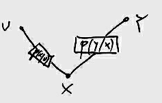
I(U, X;Y) = I(U;Y) + \cancelto0I(X;Y|U) = I(X;Y) + I(U;Y|X) → \mathchoiceI(U;Y) ≥ I(X;Y)I(U;Y) ≥ I(X;Y)I(U;Y) ≥ I(X;Y)I(U;Y) ≥ I(X;Y) во случај на идеален канал p(x|y)!!!
H(U, f(U) = H(U) + H(f(U)|U) = H(U)
Можеби треба да се оди со претпоставка дека важат маркови ланци!! На пример X1 не зависи од V ако е даден U.
iii) The receiver calculates a set L2(y(i − 1)) of z such that z ∈ L2(y(i − 1)) if (ŷ1(z|ŵi − 1, ŝi − 1, m̂i − 1), x2(ŝi − 1|m̂i − 1), y(i − 1)) are jointly ϵ-typical. The receiver declares that ẑi − 1 was sent in block i − 1 if:
From
[12] we see that
ẑi − 1 = zi − 1 with arbitrarily small probability of error if
n is sufficiently large and
I(Ŷ1;Y1|X2, U) + ϵ < I(Ŷ1;Y|X2, U) + I(X2;Y|V) − ϵ
But since
I(Ŷ1;Y1, Y|X2, U) = I(Ŷ1;Y1|X2, U)
\strikeout off\uuline off\uwave off
I(Ŷ1;Y1, Y|X2, U) = I(Ŷ1;Y1|X2, U) + \cancelto0I(Ŷ1;Y|X2, U, Y1) = I(Ŷ1;Y1|X2, U) + H(Ŷ1|X2, U, Y1) − H(Ŷ1|X2, U, Y1, Y) = I(Ŷ1;Y1|X2, U)
\strikeout off\uuline off\uwave offВеројатно нема неизвесност да го знаеш Ŷ1 ако го знаеш Y1.
Then condition
79↑ becomes
I(X2;Y|V) > I(Ŷ1;Y1|Y, X2, U) + 2ϵ
I(X2;Y|V) > I(Ŷ1;Y1|X2, U) − I(Ŷ1;Y|X2, U) + 2ϵ = I(Ŷ1;Y1, Y|X2, U) − \cancelto0I(Ŷ1;Y|X2, U) + 2ϵ = I(Ŷ1;Y1, Y|X2, U) + 2ϵ.
which as
ϵ → 0 gives condition
74↑ in Theorem 7.
iv) Using both ŷ1(ẑi − 1|ŵi − 1’, ŝi − 1, m̂i − 1) and y(i − 1), the receiver finally declares that ŵi − 1’’ was sent in block i − 1 if \strikeout off\uuline off\uwave off(x1(ŵi − 1’’|ŵi − 1’, m̂i − 1), ŷ1(ẑi − 1|ŵi − 1’, ŝi − 1, m̂i − 1), y(i − 1)) are jointly ϵ-typical. ŵi − 1’’ = wi − 1’’ with high probability if
\strikeout off\uuline off\uwave off
R1 < I(X1;Y, Ŷ1|X2)
\strikeout off\uuline off\uwave offR1 < I(V;Y) + I(U;Y|X2, V) − ϵ
and n is sufficiently large.
v) The relay upon receiving y1(i) declares that w’̂ was received if (u(w’̂|mi), y1(i), x2(si|mi)) are jointly ϵ-typical. wi’ = ŵ’ with high probability if:
and n is sufficiently large. Thus, the relay knows that wi’ ∈ S1mi + 1.
vi) The relay also estimates zi such that (ŷ1(zi|wi’, si, mi), y1(i), x2(si|mi)) are jointly ϵ-typical. Such a zi will exist with high probability for large n, therefore the relay knows that zi ∈ S2si + 1.
R1 < I(V;Y) + I(U;Y|X2, V) − ϵ
R2 = I(X1;Y, Ŷ1|X2, U) − ϵ
.
therefore, the rate of transmission from X1 to Y is bounded by:
R < I(U;Y1|X2, V) + I(X1;Y, Ŷ1|X2, V) − ϵ
ова е првиот член од минимумот во 72↑
Ова е вториот член од минимумот во 72↑
Ова ми изгледа како да зема R = R1 + R2;
Substituting from
79↑ we obtain
\strikeout off\uuline off\uwave off
I(X2;Y|V) > I(Ŷ1;Y1|X2, U) − I(Ŷ1;Y|X2, U) + 2ϵ
\strikeout off\uuline off\uwave off(a) I(X2;Y|V) > I(Ŷ1;Y1|Y, X2, U) + 2ϵ
\strikeout off\uuline off\uwave off(b) I(Ŷ1;Y1, Y|X2, U) = I(Ŷ1;Y1|X2, U)
\strikeout off\uuline off\uwave offI(Ŷ1;Y1|X2, U) + ϵ < I(Ŷ1;Y|X2, U) + I(X2;Y|V) − ϵ
\strikeout off\uuline off\uwave offR < I(V;Y) + I(U;Y|X2, V) + I(X1;Y, Ŷ1|X2, U) − 2ϵ
I(X2, V;Y) = I(V;Y) + I(X2;Y|V) → \mathchoiceI(V;Y)I(V;Y)I(V;Y)I(V;Y) = I(X2, V;Y) − I(X2;Y|V) = |(a)| < \mathchoiceI(X2, V;Y) − I(Ŷ1;Y1|Y, X2, U) − 2ϵI(X2, V;Y) − I(Ŷ1;Y1|Y, X2, U) − 2ϵI(X2, V;Y) − I(Ŷ1;Y1|Y, X2, U) − 2ϵI(X2, V;Y) − I(Ŷ1;Y1|Y, X2, U) − 2ϵ
Во
82↑ имаш \strikeout off\uuline off\uwave off
R < I(V;Y) + I(U;Y|X2, V) + I(X1;Y, Ŷ1|X2, U) − 2ϵ
R < I(X2, V;Y) − I(Ŷ1;Y1|Y, X2, U) − 2ϵ + I(U;Y|X2, V) + I(X1;Y, Ŷ1|X2, U) − 2ϵ =
= \mathchoiceI(X2, V;Y) − I(Ŷ1;Y1|Y, X2, U) + I(U;Y|X2, V) + I(X1;Y, Ŷ1|X2, U) − 4ϵI(X2, V;Y) − I(Ŷ1;Y1|Y, X2, U) + I(U;Y|X2, V) + I(X1;Y, Ŷ1|X2, U) − 4ϵI(X2, V;Y) − I(Ŷ1;Y1|Y, X2, U) + I(U;Y|X2, V) + I(X1;Y, Ŷ1|X2, U) − 4ϵI(X2, V;Y) − I(Ŷ1;Y1|Y, X2, U) + I(U;Y|X2, V) + I(X1;Y, Ŷ1|X2, U) − 4ϵ =
= I(X2, V;Y) − I(Ŷ1;Y1|Y, X2, U) + I(U;Y|X2, V) + I(X1;Y|X2, U) + I(X1;Y|X2, U, Ŷ1) − 4ϵ ???
= I(X2;Y) + I(V;Y|X2) − I(Ŷ1;Y1|Y, X2, U) + I(U;Y|X2, V) + I(X1;Y|X2, U) + I(X1;Y|X2, U, Ŷ1) − 4ϵ ???
R < I(X1, X2;Y) − I(Ŷ1;Y1|X2, X1, U, Y) − 4ϵ
\strikeout off\uuline off\uwave offI(X1Y1;Ŷ1|X2, U, Y) = \cancelto0I(X1;Ŷ1|X2, U, Y, Y1) + I(Y1;Ŷ1|X2, U, Y) = I(X1;Ŷ1|X2, U, Y) + I(Y1;Ŷ1|X1X2U, Y) →
\mathchoiceI(Y1;Ŷ1|X2, U, Y) = I(X1;Ŷ1|X2, U, Y) + I(Y1;Ŷ1|X1X2U, Y)I(Y1;Ŷ1|X2, U, Y) = I(X1;Ŷ1|X2, U, Y) + I(Y1;Ŷ1|X1X2U, Y)I(Y1;Ŷ1|X2, U, Y) = I(X1;Ŷ1|X2, U, Y) + I(Y1;Ŷ1|X1X2U, Y)I(Y1;Ŷ1|X2, U, Y) = I(X1;Ŷ1|X2, U, Y) + I(Y1;Ŷ1|X1X2U, Y)
\strikeout off\uuline off\uwave offR < I(X2, V;Y) − I(X1;Ŷ1|X2, U, Y) − I(Y1;Ŷ1|X1X2U, Y) + I(U;Y|X2, V) + I(X1;Y, Ŷ1|X2, U) − 4ϵ =
\strikeout off\uuline off\uwave off = I(X2, V;Y) − \cancelI(X1;Ŷ1|X2, U, Y) − I(Y1;Ŷ1|X1X2U, Y) + I(U;Y|X2, V) + I(X1;Y|X2, U) + \cancelI(X1;Ŷ1|X2, U, Y) − 4ϵ =
= \mathchoiceI(X2, V;Y) + I(U;Y|X2, V)I(X2, V;Y) + I(U;Y|X2, V)I(X2, V;Y) + I(U;Y|X2, V)I(X2, V;Y) + I(U;Y|X2, V) + I(X1;Y|X2, U) − I(Y1;Ŷ1|X1X2U, Y) − 4ϵ =
\strikeout off\uuline off\uwave offI(X2, V;Y) + I(U;Y|X2, V) = I(U, X2, V;Y)
= I(U, X2, V;Y) + I(X1;Y|X2, U) − I(Y1;Ŷ1|X1X2U, Y) − 4ϵ =
I(X1, X2, U;Y) = I(X1;Y|X2, U) + I(X2, U;Y) → \mathchoiceI(X1, X2, U;Y) − I(X2, U;Y) = I(X1;Y|X2, U)I(X1, X2, U;Y) − I(X2, U;Y) = I(X1;Y|X2, U)I(X1, X2, U;Y) − I(X2, U;Y) = I(X1;Y|X2, U)I(X1, X2, U;Y) − I(X2, U;Y) = I(X1;Y|X2, U)
= I(U, X2, V;Y) + I(X1, X2, U;Y) − I(X2, U;Y) − I(Y1;Ŷ1|X1X2U, Y) − 4ϵ =
\strikeout off\uuline off\uwave off = \cancelI(U, X2;Y) + I(V;Y|U, X2) + I(X1, X2, U;Y) − \cancelI(X2U;Y) − I(Y1;Ŷ1|X1X2U, Y) − 4ϵ =
= I(V;Y|U, X2) + I(X1, X2, U;Y) − I(Y1;Ŷ1|X1, X2, U, Y) − 4ϵ = I(V;Y|U, X2) + I(X1, X2;Y) + I(U;Y|X1X2) − I(Y1;Ŷ1|X1, X2, U, Y) − 4ϵ =
I(X1, X2, U;Y) = I(X1, X2;Y) + I(U;Y|X1X2) = I(X1, X2;Y) + I(X1U;Y|X2) − I(X1;Y|X2)
I(X1U;Y|X2) = I(X1;Y|X2) + I(U;Y|X1X2)
I(V;Y|U, X2) + I(U;Y|X1X2) = H(Y|U, X2) − H(Y|V, U, X2) + H(Y|X1X2) − H(Y|U, X1X2)
претпоставувам дека се работи за маркови ланци и Y не зависи од U ако е даден X1. Исто така Y не зависи од V ако е даден X2. Под ваквов услов:
\mathchoiceI(V;Y|U, X2) + I(U;Y|X1X2) = 0I(V;Y|U, X2) + I(U;Y|X1X2) = 0I(V;Y|U, X2) + I(U;Y|X1X2) = 0I(V;Y|U, X2) + I(U;Y|X1X2) = 0
= \cancelto0I(V;Y|U, X2) + I(U;Y|X1X2) + I(X1, X2;Y) − I(Y1;Ŷ1|X1, X2, U, Y) − 4ϵ = I(X1, X2;Y) − I(Y1;Ŷ1|X1, X2, U, Y) − 4ϵ докажано!!!
which establishes Theorem 7.
7 Concluding Remarks
Theorem 1,2 and 3 establish capacity for degraded, reversely degraded, and feedback relay channels. The full understanding of the relay channel may yield the capacity of the single sender single receiver network in
8↑. This will be the
information theoretic generalization of the well known maximum flow-minimum cut theorem [9].
0. Потсети се на achievability of rate од EIT (done)
1. Треба да го поминам [6] за block markovian dependence (не знам дали ова има врска со block markov encoding)
2. Треба да го поминам [7] за random binning proof.
3. Види го доказот на Lemma 2 во [14]
4. Enumeration encoding for the relay
[6]
5.
Maximum-flow minimum cut theorem [9] (done)
6. G. Kramer, I. Maric and R. D. Yates, Cooperative Communications
7. Откри како го добива R0 за деградиран Гаусов канал.
References
[1] E. C. van der Meulen, “Three-terminal communication channels,” Adv. Appl. Prob., vol. 3, pp. 120-154, 1971.
[2] E. C. van der Meulen, “Transmission of information in a T-terminal discrete memoryless channel,” Ph.D. dissertation, Dep. of Statistics, University of California, Berkeley, 1968.
[3] E. C. van der Meulen, “A survey of multi-way channels in information theory: 1961-1976,” IEEE Trans. Inform. Theory, vol. IT-23, no. 2, January 1977.
[4] H. Sato, “Information transmission through a channel with relay,” The Aloha System, University of Hawaii, Honolulu, Tech. Rep. B76-7, Mar. 1976.
[5] C. E. Shannon, “A mathematical theory of communication,” BeN Syst. Tech. J., vol. 27, pp. 379-423, July 1948.
[6] T. M. Cover and S. K. Leung-Yan-Cheong, “A rate region for the multiple-access channel with feedback,” submitted to IEEE Trans. Inform. Theory, 1976.
[7] D. Slepian and J. K. Wolf, “Noiseless coding of correlated information sources,” IEEE Trans. Inform. Theory, vol. IT-19, pp. 47 l-480, July, 1973.
[8] T. M. Cover, “A proof of the data compression theorem of Slepian and Wolf for ergodic sources,” IEEE Trans. Inform. Theory, vol. IT-22, pp. 226-278, Mar. 1975.
[9] L. R. Ford and D. R. Fulkerson, Flows in Networks, Princeton, NJ: Princeton Univ. Press, 1962.
[10] R. Ahlswede and J. Khmer, “Source coding with side information and converse for the degraded broadcast channel,” IEEE Trans. Inform. Theory, vol. IT-21, pp. 629-637, Nov. 1975.
[11] A. D. Wyner, “On source coding with side information at the decoder,” IEEE Trans. Inform. Theory, vol. IT-21, pp. 294-300, May 1975.
[12] T. Berger, “Multiterminal source coding,” Lecture notes presented at the 1977 CISM Summer School, Udine, Italy, July 18-20, 1977, Springer-Verlag.
[13] J. Wolfowitz, Coding Theorems of Information Theory, New York: Springer-Verlag, Third Ed., 1964.
[14] T. Cover, “An achievable rate region for the broadcast channel,” IEEE Trans. Inform. Theory, vol. IT-21, pp. 399-404, Jul. 1975.
Nomenclature